IMDB Movie Assignment: Start To Analysis: Part - 3

Subtask 2.4: Find the Most Popular Trios - I

After completion of the Average Rating on the previous part, let's step into finding the most popular trios among the list given in the dataset.

For Instance, consider that a Producer wants to create a movie wherein there are three lead roles. To be on the safer side, he wants to consider those actors for Trio, who have already worked together as a Trio. In the data, we have a list of names of actors that worked together in a single film as actor_1_name, actor_2_name, and actor_3_name. Now to find the best trio, we will count the total of their Facebook likes. Ones will most like will be considered the most popular.

Follow the step to perform the same task: 

movies['likes']=movies.actor_1_facebook_likes+movies.actor_2_facebook_likes+movies.actor_3_facebook_likes
movies[['likes']].head(15)
#sorting likes in ascending order
movies.sort_values(by='likes',ascending=False,inplace=True)
movies[['actor_1_name','actor_2_name','actor_3_name','likes']].head(5)

Firstly, a new column in the dataset named likes is made and the addition of all the likes of three actors is stored into the column. The procedure is followed by sorting the data in terms of ascending order just to know trios with maximum likes.

Output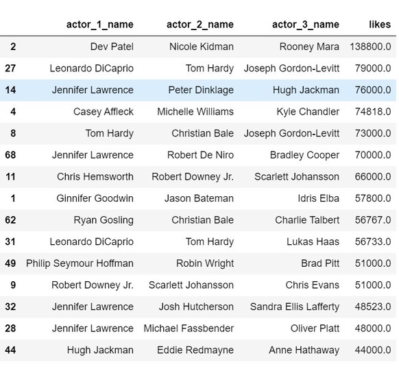

The above shown is the list of the popular trios. 

Subtask 2.5: Find the Most Popular Trios - II

Now, to consider that who among these make the best trio, the analysis will be done on a condition ie. The likes of one actor should not be less than half of the likes of the other two. To perform the same follow the code below:

act1= movies['actor_1_facebook_likes']/2
act2= movies['actor_2_facebook_likes']/2
act3= movies['actor_3_facebook_likes']/2

a=((movies['actor_1_facebook_likes'] > act1) & (movies['actor_1_facebook_likes']>act3))
b=((movies['actor_2_facebook_likes'] > act2) & (movies['actor_2_facebook_likes']>act3))
c=((movies['actor_3_facebook_likes'] > act3) & (movies['actor_3_facebook_likes']>act2))
eligible=a & b & c

movies["eligible"]=eligible
movies.loc[eligible,['eligible','actor_1_name','actor_2_name','actor_3_name']].head(5)

Output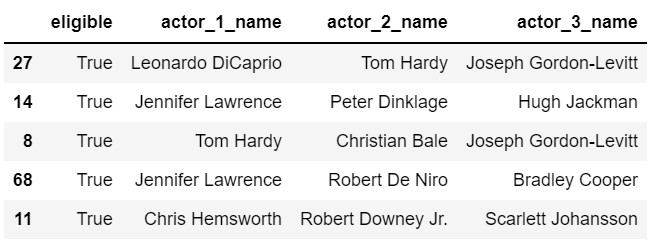

Subtask 2.6: Runtime Analysis

You can check in the dataset, there is a column named Runtime that displays the length of the movie. Let's import matplotlib and seaborn module of Python and use Displot or Histplot to see variations in the length of movies.

First, we can use distplot for the same:

import seaborn as sns
import matplotlib.pyplot as plt

sns.distplot(movies.Runtime,color='grey',rug=True,vertical=False,norm_hist=True,hist=True)
plt.show()

Output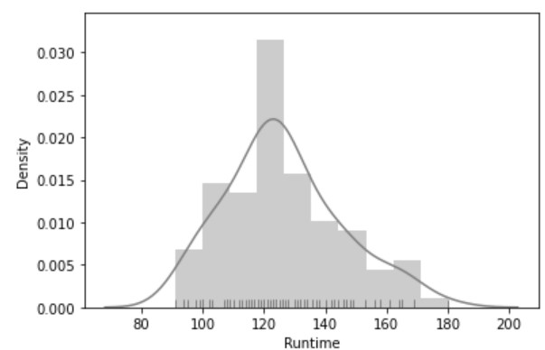

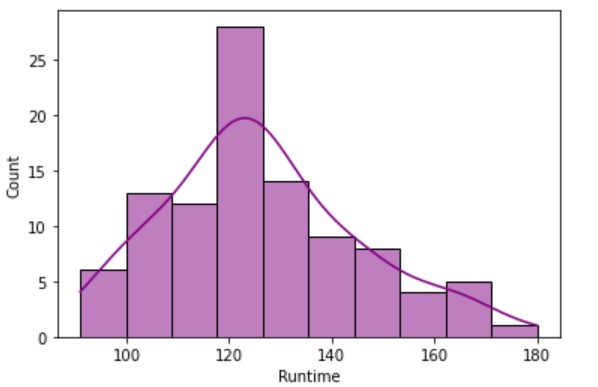
Well, this kind of plot is actually deprecated and soon will not be supported by new versions. So, we can use here Histplot as an alternative for the same analysis.

sns.histplot(x=movies.Runtime,data=movies,color='purple',fill=True,kde=True, stat='count')
plt.show()

Output

Subtask 2.7: R-Rated Movies

R-Rated movies are those movies that are restricted to under 18 groups of people. Still, the dataset contains some votes for R Rated movies from the under 18 group. 

Let's analyze which R Rated movies are voted most by under 18. CVotesU18 column represents votes of under 18 people.

PopularR=movies[(movies.content_rating=='R') & (movies.CVotesU18>0)]
PopularR.sort_values( by="CVotesU18",ascending=False,inplace=True)
PopularR[['Title']].head(10)

Output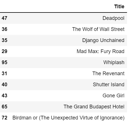

We can predict, that Deadpool is the R Rated movie that is voted most by the under 18 groups.