IMDB Movie Assignment: Demographic analysis: Part - 1

Subtask 3.1 Combine the Dataframe by Genres

Demographics Analysis means a kind of analysis based on population. There are three columns genre_1,genre_2, and genre_3 present in the dataset. let's find out other information from the data using these three columns.

1) To perform Demographics analysis, firstly let's create a dataset df_by_genre and store all the Votes and CVotes(those columns related to population) columns in it.

Follow the code below for the same:

df_by_genre=movies[['genre_1','genre_2','genre_3','CVotes10',
       'CVotes09', 'CVotes08', 'CVotes07', 'CVotes06', 'CVotes05', 'CVotes04',
       'CVotes03', 'CVotes02', 'CVotes01', 'CVotesMale', 'CVotesFemale',
       'CVotesU18', 'CVotesU18M', 'CVotesU18F', 'CVotes1829', 'CVotes1829M',
       'CVotes1829F', 'CVotes3044', 'CVotes3044M', 'CVotes3044F', 'CVotes45A',
       'CVotes45AM', 'CVotes45AF', 'CVotes1000', 'CVotesUS', 'CVotesnUS',
       'VotesM', 'VotesF', 'VotesU18', 'VotesU18M', 'VotesU18F', 'Votes1829',
       'Votes1829M', 'Votes1829F', 'Votes3044', 'Votes3044M', 'Votes3044F',
       'Votes45A', 'Votes45AM', 'Votes45AF', 'Votes1000', 'VotesUS',
       'VotesnUS']]

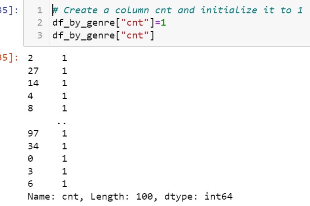
2) Moving ahead let's add a column in the dataset named cnt and initialize the column with 1. Moving further, you will realize the importance of creating a cnt column.

df_by_genre["cnt"]=1
df_by_genre["cnt"]

Output

3) After initialization of the cnt column has been done, we will group the data df_by_genre according to different genre genre_1, genre_2, and genre_3.

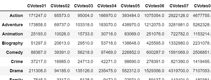
i) The data df_by_genre is grouped using genre_1 and along with that sum of all the numeric columns has been taken using sum().

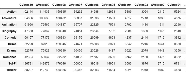
df_by_g1=df_by_genre.groupby('genre_1').sum()

Output

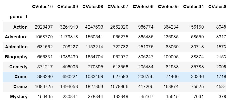
You can see that all the numerical columns based on the Action genre, have been grouped and added. The same goes for other genres.

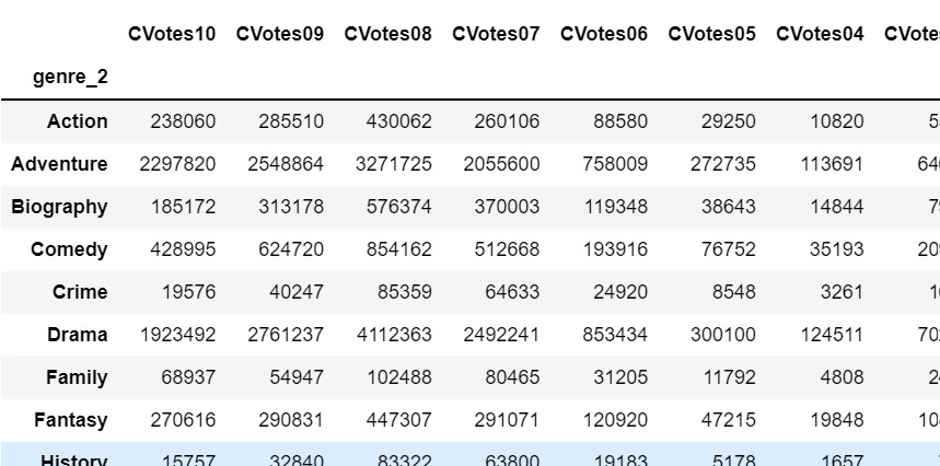
ii) Following step i) data df_by_genre will be grouped using genre_2 and genre_3 and the addition on all the numerical columns will be performed for both individually. Follow the code to perform the same:

For genre_2:

df_by_g2=df_by_genre.groupby('genre_2').sum()
df_by_g2

Output

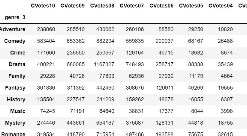
For genre_3:

df_by_g3=df_by_genre.groupby('genre_3').sum()
df_by_g3

Output

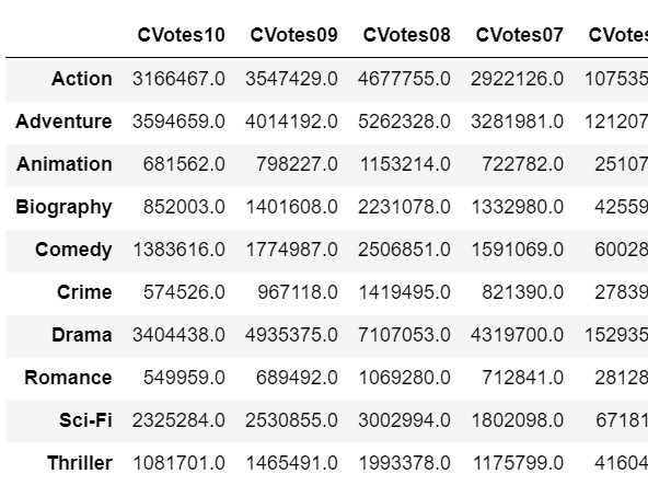
4) After the grouping of the dataset is done according to all three columns, We need to combine the output by adding numeric rows with the same genre type. Also, null values there will be replaced using 0. After combination, the result is stored into a dataset named ad df_add.

Follow the code below to perform the same task:

df_add=(df_by_g1.add(df_by_g2,axis=1,fill_value=0)).add(df_by_g3,axis=1,fill_value=0)

Output

5) If you notice cnt column, it indicates the occurrence of the individual genre after combining all 3 genre_1, genre_2, and genre_3.

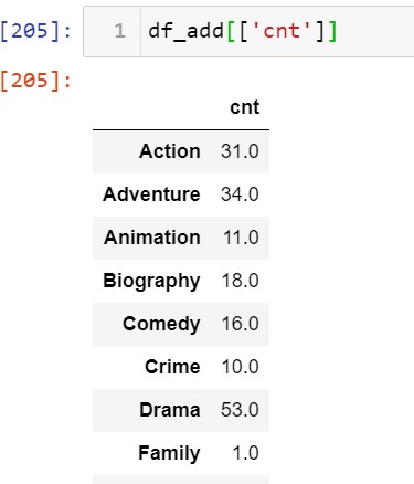
From the above output, you can conclude that Action movies are occurring 31 times individually. 

Therefore, let's find out those movies genres that have at least 10 occurrences and store the values into another dataset named genre_top10.

Follow the code to perform the above-mentioned task:

genre_top10=df_add[df_add['cnt']>=10]
genre_top10

Output

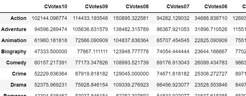
6) Moving ahead, to find the average values of all the numeric columns in genre_top10, let's find out the mean by dividing every column by cnt value. Below code is performing the same task:

# Take the mean for every column by dividing with cnt 
genre_top10[['CVotes10', 'CVotes09', 'CVotes08', 'CVotes07', 'CVotes06', 'CVotes05',
       'CVotes04', 'CVotes03', 'CVotes02', 'CVotes01', 'CVotesMale',
       'CVotesFemale', 'CVotesU18', 'CVotesU18M', 'CVotesU18F', 'CVotes1829',
       'CVotes1829M', 'CVotes1829F', 'CVotes3044', 'CVotes3044M',
       'CVotes3044F', 'CVotes45A', 'CVotes45AM', 'CVotes45AF', 'CVotes1000',
       'CVotesUS', 'CVotesnUS', 'VotesM', 'VotesF', 'VotesU18', 'VotesU18M',
       'VotesU18F', 'Votes1829', 'Votes1829M', 'Votes1829F', 'Votes3044',
       'Votes3044M', 'Votes3044F', 'Votes45A', 'Votes45AM', 'Votes45AF',
       'Votes1000', 'VotesUS', 'VotesnUS']] =genre_top10[['CVotes10',
       'CVotes09', 'CVotes08', 'CVotes07', 'CVotes06', 'CVotes05',
       'CVotes04', 'CVotes03', 'CVotes02', 'CVotes01', 'CVotesMale',
       'CVotesFemale', 'CVotesU18', 'CVotesU18M', 'CVotesU18F', 'CVotes1829',
       'CVotes1829M', 'CVotes1829F', 'CVotes3044', 'CVotes3044M',
       'CVotes3044F', 'CVotes45A', 'CVotes45AM', 'CVotes45AF', 'CVotes1000',
       'CVotesUS', 'CVotesnUS', 'VotesM', 'VotesF', 'VotesU18', 'VotesU18M',
       'VotesU18F', 'Votes1829', 'Votes1829M', 'Votes1829F', 'Votes3044',
       'Votes3044M', 'Votes3044F', 'Votes45A', 'Votes45AM', 'Votes45AF',
       'Votes1000', 'VotesUS', 'VotesnUS']].apply(lambda x: x/genre_top10.cnt)

genre_top10

Output

7) In the dataset genre_top10, you all can notice CVotes and Votes column. However, in this step of the analysis, you need to select all Votes Columns and round off all the columns up to 2 decimal places.

The code is as follows:

# Rounding off the columns of Votes to two decimals
genre_top10[['VotesM', 'VotesF', 'VotesU18', 'VotesU18M',
       'VotesU18F', 'Votes1829', 'Votes1829M', 'Votes1829F', 'Votes3044',
       'Votes3044M', 'Votes3044F', 'Votes45A', 'Votes45AM', 'Votes45AF',
       'Votes1000', 'VotesUS', 'VotesnUS']]= round(genre_top10[['VotesM', 'VotesF', 'VotesU18', 'VotesU18M',
       'VotesU18F', 'Votes1829', 'Votes1829M', 'Votes1829F', 'Votes3044',
       'Votes3044M', 'Votes3044F', 'Votes45A', 'Votes45AM', 'Votes45AF',
       'Votes1000', 'VotesUS', 'VotesnUS']],2)


genre_top10[['VotesM', 'VotesF', 'VotesU18', 'VotesU18M',
       'VotesU18F', 'Votes1829', 'Votes1829M', 'Votes1829F', 'Votes3044',
       'Votes3044M', 'Votes3044F', 'Votes45A', 'Votes45AM', 'Votes45AF',
       'Votes1000', 'VotesUS', 'VotesnUS']]

and convert all the CVotes columns from float to integer type:

genre_top10[['CVotes10', 'CVotes09', 'CVotes08', 'CVotes07', 'CVotes06', 'CVotes05',
       'CVotes04', 'CVotes03', 'CVotes02', 'CVotes01', 'CVotesMale',
       'CVotesFemale', 'CVotesU18', 'CVotesU18M', 'CVotesU18F', 'CVotes1829',
       'CVotes1829M', 'CVotes1829F', 'CVotes3044', 'CVotes3044M',
       'CVotes3044F', 'CVotes45A', 'CVotes45AM', 'CVotes45AF', 'CVotes1000',
       'CVotesUS', 'CVotesnUS']]=genre_top10[['CVotes10', 'CVotes09',
       'CVotes08', 'CVotes07', 'CVotes06', 'CVotes05',
       'CVotes04', 'CVotes03', 'CVotes02', 'CVotes01', 'CVotesMale',
       'CVotesFemale', 'CVotesU18', 'CVotesU18M', 'CVotesU18F', 'CVotes1829',
       'CVotes1829M', 'CVotes1829F', 'CVotes3044', 'CVotes3044M',
       'CVotes3044F', 'CVotes45A', 'CVotes45AM', 'CVotes45AF', 'CVotes1000',
       'CVotesUS', 'CVotesnUS']].astype('int')

genre_top10[['CVotes10', 'CVotes09', 'CVotes08', 'CVotes07', 'CVotes06', 'CVotes05',
       'CVotes04', 'CVotes03', 'CVotes02', 'CVotes01', 'CVotesMale',
       'CVotesFemale', 'CVotesU18', 'CVotesU18M', 'CVotesU18F', 'CVotes1829',
       'CVotes1829M', 'CVotes1829F', 'CVotes3044', 'CVotes3044M',
       'CVotes3044F', 'CVotes45A', 'CVotes45AM', 'CVotes45AF', 'CVotes1000',
       'CVotesUS', 'CVotesnUS']]

Output

Subtask 3.2: Genre Counts!

8) Now let's try to make some insights by plotting a bar chart for different genres Vs cnt:

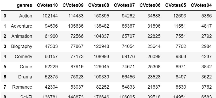
i) Firstly we need to reset the index and rename the axis. Follow the code below for the same

genre_top10=genre_top10.rename_axis('genres').reset_index()
genre_top10

Output

ii) Drafting the Bar char for Genre vs cnt will require the following code:

# barplot for genres
plt.figure(figsize=[10,7])
sns.barplot(y='genres',x='cnt',data=genre_top10,palette='twilight',lw=1,ec='white',hatch='-+')
plt.show() 

Output

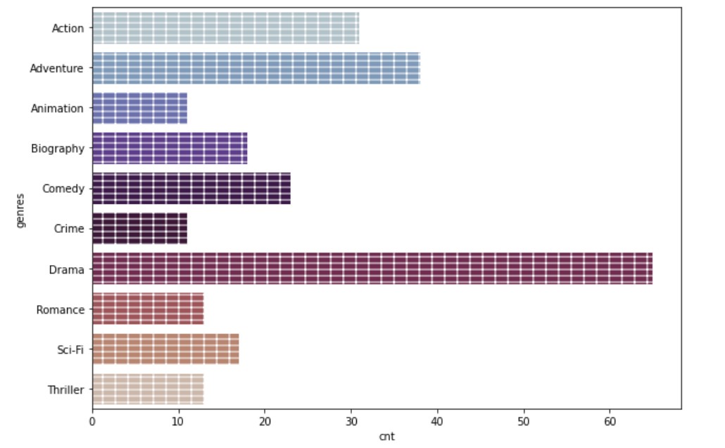
The above chart shows the tallest bar for Drama movies. Therefore, it can be concluded that movies with Drama genre are present the most.