Linear Regression Process

Here we will see the step by step calculation of Linear Regression with the help of an example.

Let's suppose that we are provided with the following data.

x	y
1	3
2	1
3	5
4	2
5	6
6	9
7	10
8	4
9	8

Plot all these data points on the graph.

graph

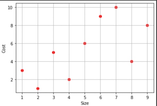
Now, our goal is to draw the regression line which passes through all these points with the least error.

Step-1: Calculate the mean of the x and y-axis.

Note: The line of regression will pass through the mean of x & y always.

Mean of x-axis=5.0

Mean of y-axis=5.34

Now we will draw a point where these two values will intersect. Thus this is the point from where our line of regression will pass.

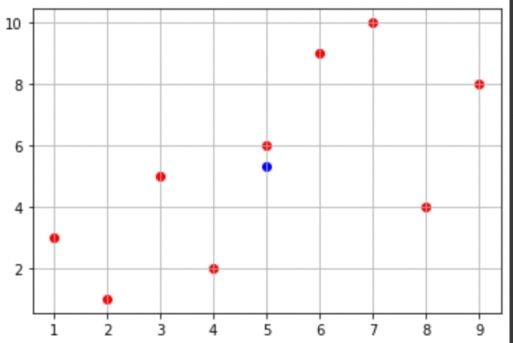
Here, the blue point is the mean value of the x and y-axis.

Step-2: Calculate the value of m

As we know the equation of a line is y=mx+c. Here

$m=\frac{\sum (x-\bar{x})\sum(y-\bar{y})}{\sum(x-\bar{x}) ^{2}}$

where (x-x̄) is nothing but the distance of all the points from x=5.

( y-ȳ)s nothing but the distance of all the points from y=5.34.

x	y	x-x̄	y-ȳ	(x-x̄)(y-ȳ)	(x-x̄)²
1	3	-4	-2.34	9.34	16
2	1	-3	-4.34	13	9
3	5	-2	-0.34	0.67	4
4	2	-1	-3.34	3.34	1
5	6	0	0.67	0	0
6	9	1	3.67	3.67	1
7	10	2	4.67	4.67	4
8	4	3	-1.34	-1.34	9
9	8	4	2.67	2.67	16

Then,

$\sum (x-\bar{x})\sum(y-\bar{y})=36$

$\sum (x-\bar{x})^{2}=60$

Therefore,

m=0.6

Step-3: Calculate the value of c

Equation of line, y=mx+c.

From the above calculations, we got

x=5, y=5.34 and m=0.6

Therefore,

5.34=5*0.6+c

c=2.34

Step-4: Find the equation of Regression Line using Equation of a line

From all the above-calculated values, we can conclude that our regression line would intersect the y-axis at 2.94 and it will also cross the point (5,5.34).

Therefore, the equation of the Regression line would be

y=0.6x+2.34.

Step-5: We will check whether the variables are dependent on independent variables or not for this process firstly we will predict the values of y.

For m=0.6,

c=2.34,

y=0.6x+2.34,

Then calculate the R² for the given data Here R² is the goodness of fit.

x	y	y-ȳ	y_p	y_p-ȳ	(y-ȳ)²	(y_p-ȳ)²
1	3	-2.34	2.94	-2.4	5.4	5.76
2	1	-4.34	3.54	-1.8	18.8	3.24
3	5	-0.34	4.14	-1.2	0.11	1.44
4	2	-3.34	4.74	-0.6	11.1	0.36
5	6	0.67	5.34	0	0.44	0
6	9	3.67	5.94	0.6	13.4	0.36
7	10	4.67	6.54	1.2	21.8	1.44
8	4	-1.34	7.14	1.8	1.7	3.24
9	8	2.67	7.74	2.4	7.1	5.76

$R^{2}=\frac{\sum (y_{p}-{y})^{2}}{\sum (y-\bar{y})^{2}}$

R² =0.27

Here, R² tends towards 0 in this case we can say that independent variables are not at all related to dependent variables. More the values of R²more will be the dependency. If we increase the value of R² the error will decrease.

graph

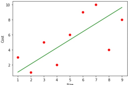
Here green line represents the line of regression.

Thu, 02/10/2022 - 08:37

Devanshi, is working as a Data Scientist with iVagus. She has expertise in Python, NumPy, Pandas and other data science technologies.