K-Prototype Clustering in Python

k-prototypes was originally proposed by Z. Huang in 1997 and was one of the earliest algorithms designed to handle mixed type data. The algorithm is initialised by randomly choosing k cluster centres, so called prototypes. For numerical and categorical data, another extension of these algorithms exists, basically combining k-means and k-modes. It is called k-prototypes i.e., the k-prototypes algorithm combines k-modes and k-means and is able to cluster mixed numerical / categorical data.

It is created in order to handle clustering algorithms with the mixed data types (numerical and categorical variables). K-Prototype is a clustering method based on partitioning. Its algorithm is an improvement of the K-Means and K-Mode clustering algorithm to handle clustering with the mixed data types.

By iteratively reallocating these prototypes to better fit the data, the algorithm tries to minimise the total distance of points assigned to a cluster and its prototype, much like the k-means algorithm. The distance function d is defined as follows for a data point x_iand a cluster prototype Q_l.

It is straightforward to integrate the k-means and k-modes algorithms into the k-prototypes algorithm that is used to cluster the mixed-type objects. The k-prototypes algorithm is practically more useful because frequently encountered objects in real world databases are mixed-type objects. The dissimilarity between two mixed-type objects X and Y , which are described by attributes A_r1, A_r2,..., A_rp, A_cp+1,..., A_cm, can be measured by

$d\left ( X_{i}Q_{l} \right )=\sum_{j=1}^{m_{r}}\left (x_{ij}^{r}q_{lj}^{r} \right )+\gamma l\sum_{j=1}^{m_{c}}\delta \left ( x_{ij}^{c}q_{lj}^{c} \right )$ Here m_r is the number of numerical attributes, mc the number of categorical objects, and $\delta$ . $\gamma l$ is a user specified parameter that describes the influence of the categorical versus numerical attributes.

$P\left ( W,Q \right )=\sum_{l=1}^{k}\left ( \sum_{i=1}^{n}w_{i,l}\sum_{j=1}^{p}\left ( x_{i,j}-q_{l,j} \right )^{2}+\gamma \sum_{i=1}^{n}w_{i,l}\sum_{j=p+1}^{m}\delta \left ( x_{i,j}-q_{l,j} \right )\right )$

let,

$P_{l}^{r}=\sum_{i=1}^{n}w_{i,l}\sum_{j=1}^{p}\left ( x_{i,j}-q_{l,j} \right )^{2}$

and

$P_{l}^{c}=\gamma \sum_{i=1}^{n}w_{i,l}\sum_{j=p+1}^{m}\delta \left ( x_{i,j}-q_{l,j} \right )$ ,

$P\left ( W,Q \right )=\sum_{l=1}^{k}\left ( P_{l}^{c} + P_{l}^{r}\right )$

Since both $P_{l}^{c} , P_{l}^{r}$ are nonnegative, minimising P(W, Q) is equivalent to minimising $P_{l}^{c} , P_{l}^{r}$ for 1 ≤ l ≤ k.

This distance measure is thus a linear combination of the Euclidean measure and the simple matching coefficient. The algorithm can be described in a few steps:

Randomly select k initial prototypes from the dataset, one for each cluster.
Allocate each data point to the cluster whose prototype is nearest to it. Update the prototype of the corresponding cluster after each allocation to be the new centre of the data in the cluster.
When all data points are assigned to a cluster, recalculate the similarity of all objects against the current prototypes. If an object is found to be nearer another prototype than the one of the cluster it belongs to, reallocate to that cluster and update the prototypes of both clusters.
Repeat steps (2-3) until convergence (i.e. no data point changes cluster).

where the first term is the squared Euclidean distance measure on the numeric attributes and the second term is the simple matching dissimilarity measure on the categorical attributes. The weight γ is used to avoid favouring either type of attribute.

For the implementation of its algorithm, the researcher needs to filter the columns carefully especially for the categorical variables. The categorical variables must be relevant to the analysis which is not meaningless information. Besides that, the quality of the input (data) affects the clustering result (cluster initialization) and how the algorithm processes the data to get the converged result. As the researcher, for the final task, interpretation, we need to consider the metrics to use for both numerical and categorical variables.

The k-prototypes algorithm has a parameter γ that controls the relative effect that the numeric and categorical attributes have on the total distance, as follows:

$d_{tot}= d_{numeric}+\gamma d_{categorical}$

In the k-prototypes algorithm, the number of clusters k can also be considered a parameter as it has to be specified by the user. A knee-plot is a common way to find the optimal number of clusters. This approach was therefore taken in this project. Since the results of k-means can vary greatly depending on initialisation, the average over four trials for each value of $\gamma$ was used for the knee plot (giving a total of 16 trials). This was done using the values $\gamma = 0.1,1,5,20$

The results of k-prototypes are evaluated using the relative-criteria approach. The validity index used is the one built-in to the k-modes package, namely the total in-cluster distance. The distance between numerical attributes is measured with the Euclidean distance and the distance in categorical attributes is the sum of the simple matching coefficient multiplied with gamma. The CV value was also used to measure the results of the k-prototype algorithm.

graph

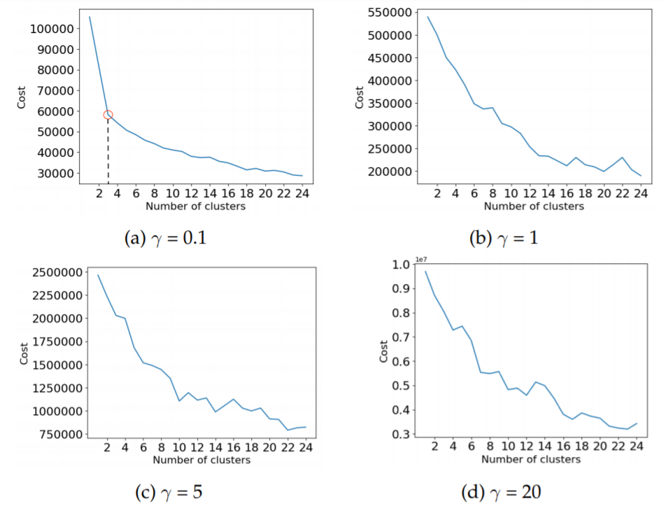
Cost as a function of the number of clusters, for different values of γ. Here on the dataset "Nulls to mean".

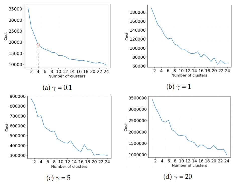
knee-plots for different values of $\gamma \left ( \gamma = 0.1,1,5,20 \right )$ , for the two different approaches to handle null values, i.e. "Nulls to mean" and "Filtered nulls", respectively. The same plots for random data. In the random data the cost is smoothly decreasing with a larger number of clusters, it does not appear to be a knee for any cluster number. Similarly, for both the "Nulls to mean" and "Filtered nulls" datasets, $\gamma = 1,5,20$ does not show any clear knees. For γ = 0.1 however, both datasets show a clear knee for 3 and 4 clusters respectively, marked with a red circle. The value $\gamma = 0.1$ was therefore chosen as the optimal value of this parameter.

it can be observed that the different numerical attributes have a spread over different values in different clusters. In contrast, many of the categories have the same value over some or all of the clusters. The corresponding validity indices for these results was a cost (total in-cluster distance) of 58000 and the CV value of 1.25.

graph

Cluster centres from k-prototypes for the seven numerical (N0-N6) and six categorical (C0-C5) features, using $\gamma = 0.1$ . The categorical feature names have been replaced by integers due to secrecy.

attribute	cluster 0	cluster 1	cluster 2
N0	32.8	7.8	5.1
N1	34.7	8.8	5.2
N2	13619477.7	614416.5	88057.3
N3	71755.7	27335.8	1229.3
N4	1311.8	119190.9	121.5
N5	23.3	11.2	15.2
N6	343.3	244.9	470.4
C0	1	2	3
C1	5	5	7
C2	1	1	1
C3	49	49	53
C4	1	1	1
C5	1	1	1
portion of data points	10%	67%	23%

The last column shows the proportion of the data points that have been assigned to each cluster. Here on the "Nulls to mean" dataset.

graph

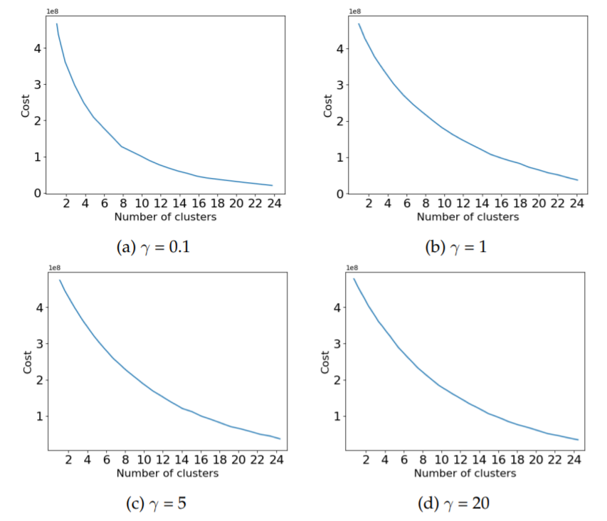
Cost as a function of the number of clusters, for different values of $\gamma$ . Here on the random data.