K-means Clustering: Centroid

The K-means clustering technique is simple, and we begin with a description of the basic algorithm. We first choose K initial centroids, where K is a user-specified parameter, namely, the number of clusters desired. Each point is then assigned to the closest centroid, and each collection of points assigned to a centroid is a cluster. The centroid of each cluster is then updated based on the points assigned to the cluster. We repeat the assignment and update steps until no point changes clusters, or equivalently, until the centroids remain the same. K-means is formally described by Algorithm. The centroids are indicated by the “+” symbol; all points belonging to the same cluster have the same marker shape.

k-means is a simple, yet often effective, approach to clustering. Traditionally, k data points from a given dataset are randomly chosen as cluster centers, or centroids, and all training instances are plotted and added to the closest cluster. After all instances have been added to clusters, the centroids, representing the mean of the instances of each cluster are re-calculated, with these re-calculated centroids becoming the new centers of their respective clusters.

At this point, all cluster membership is reset, and all instances of the training set are re-plotted and re-added to their closest, possibly re-centered, cluster. This iterative process continues until there is no change to the centroids or their membership, and the clusters are considered settled.

K-means clustering uses “centroids”, K different randomly-initiated points in the data, and assigns every data point to the nearest centroid. After every point has been assigned, the centroid is moved to the average of all of the points assigned to it. Then the process repeats: every point is assigned to its nearest centroid, centroids are moved to the average of points assigned to it.

Basic K-means algorithm.

Initialize K random centroids.
- You could pick K random data points and make those your starting points.
- Otherwise, you pick K random values for each variable.
For every data point, look at which centroid is nearest to it.
- Using some sort of measurement like Euclidean or Cosine distance.
Assign the data point to the nearest centroid.
For every centroid, move the centroid to the average of the points assigned to that centroid.
Repeat the last three steps until the centroid assignment no longer changes.
- The algorithm is said to have “converged” once there are no more changes.

Note: D(x)D(x) should be updated as more centroids are added. It should be set to be the distance between a data point and the nearest centroid.

k means

The k-means clustering algorithm attempts to split a given anonymous data set (a set containing no information as to class identity) into a fixed number (k) of clusters.

Initially k number of so called centroids are chosen. A centroid is a data point (imaginary or real) at the center of a cluster. In Praat each centroid is an existing data point in the given input data set, picked at random, such that all centroids are unique (that is, for all centroids c_i and c_j, c_i ≠ c_j). These centroids are used to train a kNN classifier. The resulting classifier is used to classify (using k = 1) the data and thereby produce an initial randomized set of clusters. Each centroid is thereafter set to the arithmetic mean of the cluster it defines. The process of classification and centroid adjustment is repeated until the values of the centroids stabilize. The final centroids will be used to produce the final classification/clustering of the input data, effectively turning the set of initially anonymous data points into a set of data points, each with a class identity.

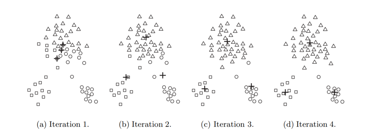
In the first step, shown in iteration 1, points are assigned to the initial centroids, which are all in the larger group of points. For this example, we use the mean as the centroid. After points are assigned to a centroid, the centroid is then updated. Again, the figure for each step shows the centroid at the beginning of the step and the assignment of points to those centroids.

In the second step, points are assigned to the updated centroids, and the centroids are updated again. In steps 2, 3, and 4, which are shown in iteration 2,3 and 4, respectively, two of the centroids move to the two small groups of points at the bottom of the figures. When the K-means algorithm terminates in iteration 4, because no more changes occur, the centroids have identified the natural groupings of points.

For some combinations of proximity functions and types of centroids, K-means always converges to a solution; i.e., K-means reaches a state in which no points are shifting from one cluster to another, and hence, the centroids don’t change. Because most of the convergence occurs in the early steps.

EUCLIDEAN CASE

Each cluster has a well defined centroid
average across all the points in the cluster
Represent each cluster by its centroid
Distance between clusters = distance between centroids

Calculate new centroid values

After each data point is assigned to a cluster, reassign the centroid value for each cluster to be the mean value of all the data points within the cluster.

$m_{i}^{t+1}= \frac{1}{\left | S_{i}^{\left ( t \right )} \right |}\sum_{x_{j}\epsilon S_{i}^{\left ( t \right )}}^{} x_{j}$

Choosing the initial centroid values

Before we discuss how to initialize centroids for k-means clustering, we must first decide how many clusters to partition the data into.

Elbow method

One method would be to try many different values of kk and plot the average distance of data points from their respective centroid (average within-cluster sum of squares) as a function of kk. This will give you something along the lines of what is shown below. Notice how increasing the kk value from 1 to 2 drastically lowers the average distance of each data point to its respective centroid, but as you continue increasing kk the improvements begin to decrease asymptotically. The ideal kk value is found at the elbow of such a plot.

Silhouette analysis

Another more automated approach would be to build a collection of k-means clustering models with a range of values for kk and then evaluate each model to determine the optimal number of clusters. We can use Silhouette analysis to evaluate each model. A Silhouette coefficient is calculated for observation, which is then averaged to determine the Silhouette score.

The coefficient combines the average within-cluster distance with average nearest-cluster distance to assign a value between -1 and 1. A value below zero denotes that the observation is probably in the wrong cluster and a value closer to 1 denotes that the observation is a great fit for the cluster and clearly separated from other clusters. This coefficient essentially measures how close an observation is to neighboring clusters, where it is desirable to be the maximum distance possible from neighboring clusters.

Centroid initialization

Once you've selected how many groups you'd like to partition your data into, there are a few options for picking initial centroid values. The simplest method? Select kk random points from your data set and call it a day. However, it's important to remember that k-means clustering results in an approximate solution converging to a local optimum - so it's possible that starting with a poor selection of centroids could mess up your clustering (ie. selecting an outlier as a centroid). The common solution to this is to run the clustering algorithm multiple times and select the initial values which end up with the best clustering performance (measured by minimum average distance to centroids - typically using within-cluster sum of squares). You can specify the number of random initializations to perform for a K-means clustering model in sci-kit learn using the n_init parameter.

random data points: In this approach, described in the "traditional" case above, k random data points are selected from the dataset and used as the initial centroids, an approach which is obviously highly volatile and provides for a scenario where the selected centroids are not well positioned throughout the entire data space.
k-means++: As spreading out the initial centroids is thought to be a worthy goal, k-means++ pursues this by assigning the first centroid to the location of a randomly selected data point, and then choosing the subsequent centroids from the remaining data points based on a probability proportional to the squared distance away from a given point's nearest existing centroid. The effect is an attempt to push the centroids as far from one another as possible, covering as much of the occupied data space as they can from initialization.
naive sharding: centroid initialization method was the subject of some of my own graduate research. It is primarily dependent on the calculation of a composite summation value reflecting all of the attribute values of an instance. Once this composite value is computed, it is used to sort the instances of the dataset. The dataset is then horizontally split into k pieces, or shards. Finally, the original attributes of each shard are independently summed, their mean is computed, and the resultant collection of rows of shard attribute mean values becomes the set of centroids to be used for initialization. The expectation is that, as a deterministic method, it should perform much quicker than stochastic methods, and approximate the spread of initial centroids across the data space via the composite summation value.

Cluster analysis

Cluster analysis is a method of organizing data into representative groups based upon similar characteristics. Each member of the cluster has more in common with other members of the same cluster than with members of the other groups. The most representative point within the group is called the centroid. Usually, this is the mean of the values of the points of data in the cluster.

Organize the data. If the data consists of a single variable, a histogram might be appropriate. If two variables are involved, graph the data on a coordinate plane. For example, if you were looking at the height and weight of school children in a classroom, plot the points of data for each child on a graph, with the weight being the horizontal axis and the height being the vertical axis. If more than two variables are involved, matrices may be needed to display the data.

Group the data into clusters. Each cluster should consist of the points of data closest to it. In the height and weight example, group any points of data that appear to be close together. The number of clusters, and whether every point of data has to be in a cluster, may depend upon the purposes of the study.

For each cluster, add the values of all members. For example, if a cluster of data consisted of the points (80, 56), (75, 53), (60, 50), and (68,54), the sum of the values would be (283, 213). Divide the total by the number of members of the cluster. In the example above, 283 divided by four is 70.75, and 213 divided by four is 53.25, so the centroid of the cluster is (70.75, 53.25). Plot the cluster centroids and determine whether any points are closer to a centroid of another cluster than they are to the centroid of their own cluster. If any points are closer to a different centroid, redistribute them to the cluster containing the closer centroid. Repeat Steps 3, 4 and 5 until all points of data are in the cluster containing the centroid to which they are closest.