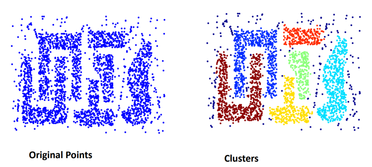
Introduction to DB Scan Clustering

Clusters are dense regions in the data space, separated by regions of lower object density. A cluster is defined as a maximal set of density connected points. Discovers clusters of arbitrary shape.

Density based clustering algorithm has played a vital role in finding non linear shapes structure based on the density. Density-Based Spatial Clustering of Applications with Noise (DBSCAN) is most widely used density based algorithm. It uses the concept of density reachability and density connectivity.

$\varepsilon$ -Neighborhood – Objects within a radius of $\varepsilon$ from an object.

$N_{\varepsilon } : \left \{ q|d\left (p,q\right )\leq \varepsilon \right \}$

“High density” - $\varepsilon$ -Neighborhood of an object contains at least MinPts of objects.

Density Reachability - An object q is directly density-reachable from object p if p is a core object and q is in p’s $\varepsilon$ -neighborhood. A point "p" is said to be density reachable from a point "q" if point "p" is within $\varepsilon$ distance from point "q" and "q" has sufficient number of points in its neighbors which are within distance $\varepsilon$ .

dbscan

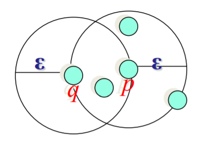
Minpts = 4

q is directly density-reachable from p
p is not directly density-reachable from q
Density-reachability is asymmetric

Density-Reachable (directly and indirectly):

A point p is directly density-reachable from p2.
p2 is directly density-reachable from p1.
p1 is directly density-reachable from q.
p $\leftarrow$ p2 $\leftarrow$ p1 $\leftarrow$ q form a chain
p is (indirectly) density-reachable from q
q is not density-reachable from p

dbscan

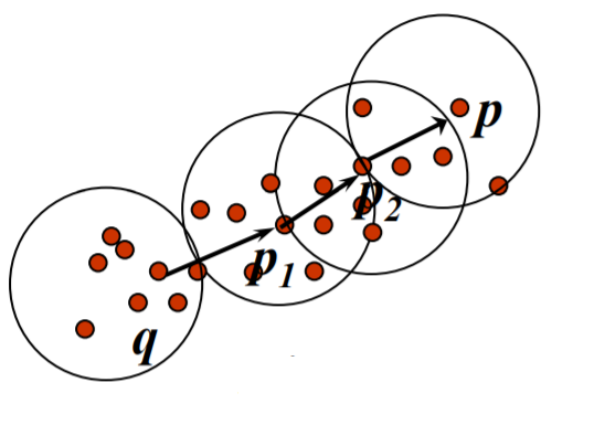
Minpts = 7

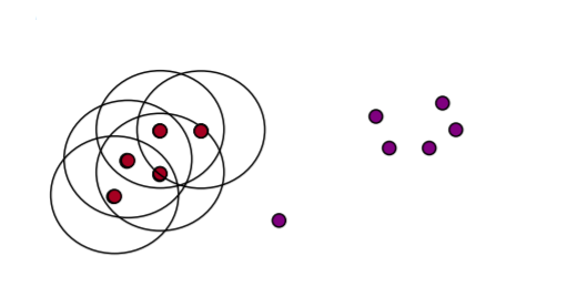
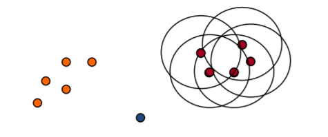
Density Connectivity - A point "p" and "q" are said to be density connected if there exist a point "r" which has sufficient number of points in its neighbors and both the points "p" and "q" are within the $\varepsilon$ distance. This is chaining process. So, if "q" is neighbor of "r", "r" is neighbor of "s", "s" is neighbor of "t" which in turn is neighbor of "p" implies that "q" is neighbor of "p".

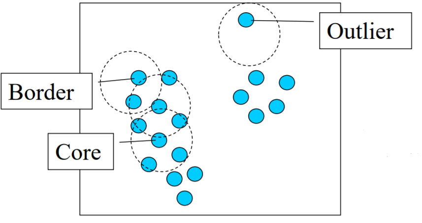
Core, Border & Outlier

Given $\varepsilon$ = 1 unit and MinPts = 5, categorize the objects into three exclusive groups.

A point is a core point if it has more than a specified number of points (MinPts) within Eps. These are points that are at the interior of a cluster. A border point has fewer than MinPts within Eps, but is in the neighborhood of a core point. A noise point is any point that is not a core point nor a border point.

A set r is a core point iff the ϵ-neighborhood ofr contains at least minPts sets:r is core ⇔ |Nϵ (r)| ≥ minPts. A sets is a border point iff it is in the ϵ-neighborhood of a core point r and s is not core:s is border ⇔ s ∈ Nϵ (r)∧ |Nϵ (r) | ≥ minPts∧ |Nϵ (s) | < minPts. All remaining sets in R are noise. We denote the set of core and border points with C and B, respectively. The set of noise points is N = R \ (C ∪ B)

dbscan

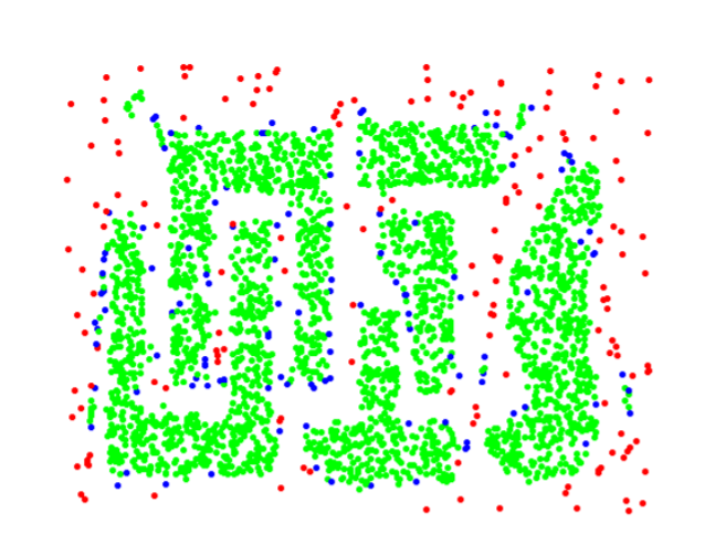
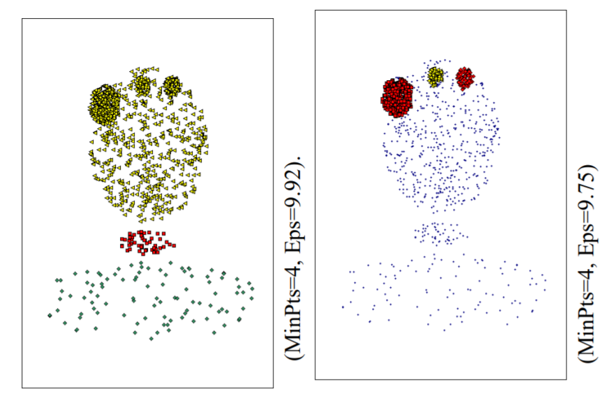
Examples: $\varepsilon$ = 10, MinPts = 4

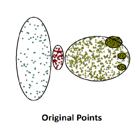
original points -

dbscan

Point types: core, border and outliers

dbscan

DBSCAN Algorithm

The standard DBSCAN algorithm forms clusters by repeatedly picking a seed point from the set of unvisited data points (initially all points are unvisited). If the seed is a core point, it forms a new cluster with all points that are density-reachable from the seed and are not yet assigned to a cluster. The set of density-reachable points is computed by recursively adding the $\varepsilon$ -neighbors of all core points to the current cluster. The algorithm terminates when all points have been visited. Points that cannot be assigned to a cluster are noise.

Algorithmic steps for DBSCAN clustering

Let X = {x₁, x₂, x₃, ..., x_n} be the set of data points. DBSCAN requires two parameters: ε (eps) and the minimum number of points required to form a cluster (minPts).

Start with an arbitrary starting point that has not been visited.
Extract the neighborhood of this point using ε (All points which are within the ε distance are neighborhood).
If there are sufficient neighborhood around this point then clustering process starts and point is marked as visited else this point is labeled as noise (Later this point can become the part of the cluster).
If a point is found to be a part of the cluster then its ε neighborhood is also the part of the cluster and the above procedure from step 2 is repeated for all ε neighborhood points. This is repeated until all points in the cluster is determined.
A new unvisited point is retrieved and processed, leading to the discovery of a further cluster or noise.
This process continues until all points are marked as visited.

Examples

1. Parameter :

$\varepsilon$ = 2 cm and
MinPts = 3

dbscan

for each o  D do                                                                                                                                                
  if o is not yet classified then                                                                                                                             
      if o is a core-object then                                                                                                                               
            collect all objects density-reachable from o                                                                                            
            and assign them to a new cluster.                                                                                                          
      else                                                                                                                                                               
            assign o to NOISE

2. Parameter

$\varepsilon$ = 2 cm
MinPts = 3

dbscan

or each o  D do                                                                                                                                                
  if o is not yet classified then                                                                                                                             
      if o is a core-object then                                                                                                                               
            collect all objects density-reachable from o                                                                                            
            and assign them to a new cluster.                                                                                                          
      else                                                                                                                                                               
            assign o to NOISE

Determining EPS and MinPts

Idea is that for points in a cluster, their kth nearest neighbors are at roughly the same distance
Noise points have the kth nearest neighbor at farther distance
So, plot sorted distance of every point to its kth nearest neighbor

When DBSCAN Works Well

Resistant to Noise
Can handle clusters of different shapes and sizes

dbscan

When DBSCAN Does NOT Work Well

Cannot handle varying densities
sensitive to parameters hard to determine the correct set of parameters

dbscan

Advantages

1) Does not require a-priori specification of number of clusters.

2) Able to identify noise data while clustering.

3) DBSCAN algorithm is able to find arbitrarily size and arbitrarily shaped clusters.

Disadvantages

1) DBSCAN algorithm fails in case of varying density clusters.

2) Fails in case of neck type of dataset.