IMDB Movie Assignment: Demographic analysis: Part - 2

Subtask 3.3: Gender and Genre

In this part of the Case Study, we can notice in the CVotes and Votes columns we have the suffix as M and F that specifies gender as Male and female. Now, let's identify the popularity of different genres among the two genders of different age groups. To do this, the concept of the heatmap in seaborn will be followed:

Analysis based on CVotes:

1) Firstly you need to create two datasets:

• male that contains all CVotes columns of the different age groups for the male gender.
• female that contains all CVotes columns of the different age groups for the female gender.

male= genre_top10[["genres","CVotesU18M","CVotes1829M","CVotes3044M","CVotes45AM"]]
female=genre_top10[["genres","CVotesU18F","CVotes1829F","CVotes3044F","CVotes45AF"]]

NOTE: Although the genres column is not related to CVotes, the column is added in both of the datasets male and female because you need to set those values of the genre as the index of the dataset.

 2) Secondly, to set the x-axis according to different age group columns and y-axis as different genres, You need to set genres as index values in both the dataset male and female:

male.set_index(['genres'], inplace = True)
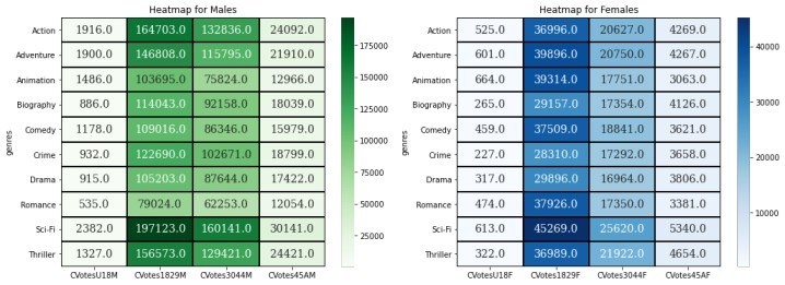
female.set_index(['genres'], inplace = True)

 3) To drive insight for both the male and female gender individually, the visualization will be done using a heatmap of Seaborn. The first heatmap will be drafted to see how different age groups of males will vary along with different genres. Then, the second heatmap will be drafted in the same way for females. 

Also, You are going to see how both the heatmaps will be drawn side by side to draw clear insight between males and females. We are going to do this with the help of Subplots:

fig, ax =plt.subplots(1,2,figsize=[17,6])
sns.heatmap(male,
            cmap='Greens', 
            annot=True,
            fmt='.1f',
            annot_kws={
                'fontsize':14,
                'fontfamily':'Serif'},
            linewidth=1,
            linecolor='black',
            ax=ax[0])

sns.heatmap(female,
            cmap='Blues', 
            annot=True,
            fmt='.1f',
            annot_kws={
                'fontsize':14,
                'fontfamily':'Serif'},
            linewidth=1,
            linecolor='black',
            ax=ax[1]
           )
ax[0].set_title('Heatmap for Males')
ax[1].set_title('Heatmap for Females')
plt.show()

OUTPUT:

Similarly, the analysis will be done for Votes columns. Follow below for the same:

Analysis based on Votes Columns:

1) This is the step for the creation of 2 datasets and setting index for the database:

• Votes_male contains all Votes columns of the different age groups for the male gender.
• Votes_male contains all Votes columns of the different age groups for the female gender.

Votes_male=genre_top10[["genres","VotesU18M","Votes1829M","Votes3044M","Votes45AM"]]
Votes_female=genre_top10[["genres","VotesU18F","Votes1829F","Votes3044F","Votes45AF"]]
Votes_male.set_index(['genres'], inplace = True)
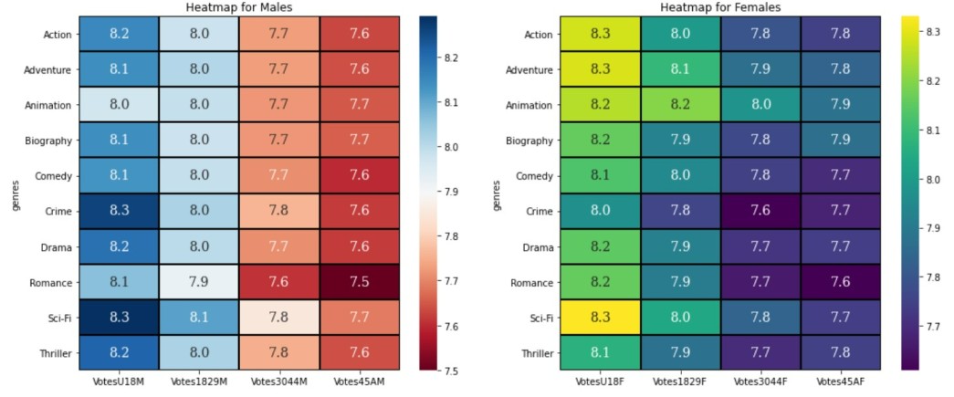
Votes_female.set_index(['genres'], inplace = True)

2) Now, plotting the heatmaps for Votes Columns as did for CVotes, follow the code below:

fig, ax =plt.subplots(1,2,figsize=[17,7])
sns.heatmap(Votes_male,
            cmap='RdBu', 
            annot=True,
            fmt='.1f',
            annot_kws={
                'fontsize':14,
                'fontfamily':'Serif'},
            linewidth=1,
            linecolor='black',
            ax=ax[0])

sns.heatmap(Votes_female,
            cmap='viridis', 
            annot=True,
            fmt='.1f',
            annot_kws={
                'fontsize':14,
                'fontfamily':'Serif'},
            linewidth=1,
            linecolor='black',
            ax=ax[1]
           )
ax[0].set_title('Heatmap for Males')
ax[1].set_title('Heatmap for Females')
plt.show()

OUTPUT: