A Dendrogram is a diagram that represents the hierarchical relationship between objects. The Dendrogram is used to display the distance between each pair of sequentially merged objects.
These are commonly used in studying hierarchical clusters before deciding the number of clusters significant to the dataset. The distance at which the two clusters combine is referred to as the dendrogram distance. The primary use of a dendrogram is to work out the best way to allocate objects to clusters. The key point to interpreting or implementing a dendrogram is to focus on the closest objects in the dataset.
Note:-
- Distance between data points represents dissimilarities.
- Height of the blocks represents the distance between clusters.
Hence from the above figure, we can observe that the objects P6 and P5 are very close to each other, merging them into one cluster named C1, and followed by the object P4 is closed to the cluster C1, so combine these into a cluster (C2). And the objects P1 and P2 are close to each other so merge them into one cluster (C3), now cluster C3 is merged with the following object P0 and forms a cluster (C4), the object P3 is merged with the cluster C2, and finally the cluster C2 and C4 and merged into a single cluster (C6).
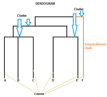
A dendrogram can be a column graph (as in the image below) or a row graph. Some dendrograms are circular or have a fluid-shape, but the software will usually produce a row or column graph. No matter what the shape, the basic graph comprises the same parts:
- The Clades are the branch and are arranged according to how similar (or dissimilar) they are. Clades that are close to the same height are similar to each other; clades with different heights are dissimilar — the greater the difference in height, the more dissimilarity.
- Each clade has one or more leaves.
- Leaves A, B, and C are more similar to each other than they are to leaves D, E, or F.
- Leaves D and E are more similar to each other than they are to leaves A, B, C, or F.
- Leaf F is substantially different from all of the other leaves.
A clade can theoretically have an infinite amount of leaves. However, the more leaves you have, the harder the graph will be to read with the naked eye.
Role of Dendrograms for Hierarchical Clustering
once one large cluster is formed by the combination of small clusters, dendrograms of the cluster are used to actually split the cluster into multiple clusters of related data points. A dendrogram is a type of tree diagram showing hierarchical clustering relationships between similar sets of data. They are frequently used in biology to show clustering between genes or samples, but they can represent any type of grouped data.
Parts of a Dendrogram
A dendrogram can be a column graph (as in the image below) or a row graph. Some dendograms are circular or have a fluid-shape, but software will usually produce a row or column graph. No matter what the shape, the basic graph comprises of the same parts:
- The clade is the branch. Usually labeled with Greek letters from left to right (e.g. α β, δ…).
- Each clade has one or more leaves. The leaves in the above image are:
- Single (simplicifolius): F
- Double (bifolius): D E
- Triple (trifolious): A B C
A clade can theoretically have an infinite amount of leaves. However, the more leaves you have, the harder the graph will be to read with the naked eye.
Plotting a Dendrogram
A dendrogram is a visualization in form of a tree showing the order and distances of merges during the hierarchical clustering.
# calculate full dendrogram
plt.figure(figsize=(25, 10))
plt.title('Hierarchical Clustering Dendrogram')
plt.xlabel('sample index')
plt.ylabel('distance')
dendrogram(
    Z,
    leaf_rotation=90.,  # rotates the x axis labels
    leaf_font_size=8.,  # font size for the x axis labels
)
plt.show()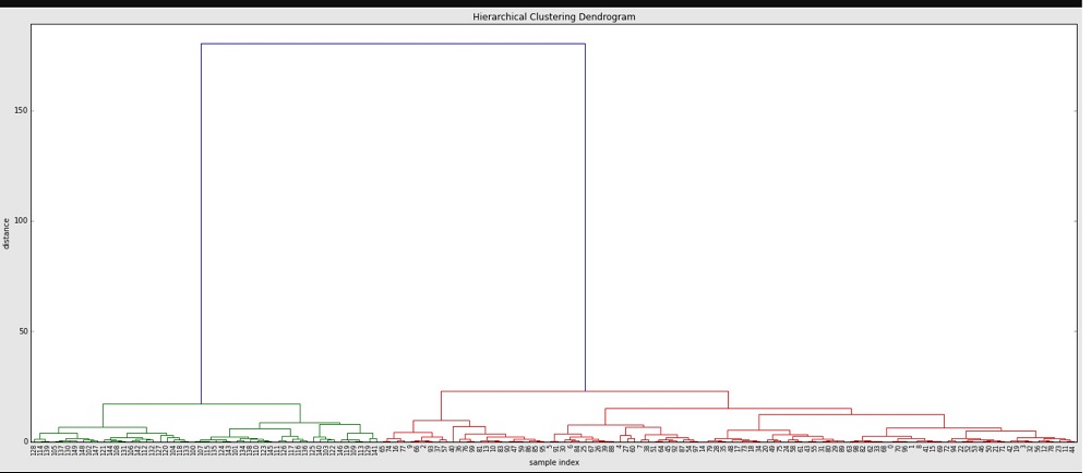
- On the x axis you see labels. If you don't specify anything else they are the indices of your samples in X.
- On the y axis you see the distances (of the 'ward' method in our case).
Starting from each label at the bottom, a vertical line up to a horizontal line. The height of that horizontal line tells about the distance at which this label was merged into another label or cluster. Other cluster by following the other vertical line down again. If you don't encounter another horizontal line, it was just merged with the other label you reach, otherwise it was merged into another cluster that was formed earlier.
- horizontal lines are cluster merges
- vertical lines tell you which clusters/labels were part of merge forming that new cluster
- heights of the horizontal lines tell you about the distance that needed to be "bridged" to form the new cluster
You can also see that from distances > 25 up there's a huge jump of the distance to the final merge at a distance of approx. 180. Let's have a look at the distances of the last 4 merges:
In [13]:
Z[-4:,2]Out[13]:
array([ 15.11533, 17.11527, 23.12199, 180.27043])Looking at indices in the above dendrogram also shows us that the green cluster only has indices >= 100, while the red one only has such < 100.
How to Read a Dendrogram
The clades are arranged according to how similar (or dissimilar) they are. Clades that are close to the same height are similar to each other; clades with different heights are dissimilar the greater the difference in height, the more dissimilarity (you can measure similarity in many different ways; One of the most popular measures is Pearson’s Correlation Coefficient).
- Leaves A, B, and C are more similar to each other than they are to leaves D, E, or F.
- Leaves D and E are more similar to each other than they are to leaves A, B, C, or F.
- Leaf F is substantially different from all of the other leaves.
the same clave, β joins leaves A, B, C, D,and E. That means that the two groups (A,B,C & D,E) are more similar to each other than they are to F.
Principal types of dendrogram
1.) A first major characteristic of dendrograms, as has already been noted, is whether they are binary or not. There are precisely n - 1 non-terminal nodes in a binary dendrogram. Many clustering programs output dendrograms in this form (e.g. the widely used CLUSTAN package), and most of the dendrograms to be discussed fall into the binary category.
2.) A second characteristic of dendrograms is whether or not the terminal nodes are labelled.
3.) A third characteristic is whether or not ranks (or level values) are associated with the nodes of the dendrogram. Either the rank values of clusters, or alternatively only the embedded or nested structure of clusters, are taken into account.
This breakdown of dendrograms between ranked and non-ranked is the same as locally or globally order invariant.
For binary dendrograms we will review the following cases: -
- labelled, ranked (L-R),
- labelled, non-ranked (L-NR),
- unlabelled, non-ranked (NL-NR),
- unlabelled, ranked (NL-R)
and for non-binary dendrograms, results will be given for: -
- labelled
- ranked
- labelled
- non-ranked.
Finally a type of binary dendrogram which will be called quasi-labelled, non-ranked.
How Dendrogram works
To visualize the dendrogram, we’ll use the following R functions and packages:
- fviz_dend()[in factoextra R package] to create easily a ggplot2-based beautiful dendrogram.
- dendextend package to manipulate dendrograms
Before continuing, install the required package as follow:
install.packages(c("factoextra", "dendextend"))- The program first computes the distances between each pair of classes in the input signature file.
- it iteratively merges the closest pair of classes and successively merges the next closest pair of classes and the succeeding closest until the classes are all merged.
- After each merging, the distances between all pairs of classes are updated. The distances at which the signatures of classes are merged are used to construct a dendrogram.
When the Use variance in distance calculations option is unchecked (MEAN_ONLY in Python), the distance dmn between a pair of classes m and n is measured as a distance between their means:
where:
m and n—The IDs of classes
i—A layer number
µ—A mean of class m or n in layer i
When the variance option is checked (VARIANCE in Python), the Dendrogram tool measures distances between pairs of classes based on their means and variances using the following formula:
where V is a variance of a class m or n in layer i.
The two signatures used to create the merged class are replaced by a single signature of the combined class. The new mean signature is computed based on the locations in the multidimensional attribute space of all member cells of the merged class.
The new means and variances describe the merged class which are based on the original mean and variance of the samples that comprise the merged class. Therefore, the merged class is produced using the pooled mean and variance. The new mean signature is computed based on the locations in the multidimensional attribute space of all member cells of the merged class.
The new signature retains the lower number of the two input classes for the merged class ID. The two signatures used to create the merged class are replaced by a single signature of the combined class.
Manipulating dendrograms using 'dendextend'
The dendextend package provides a flexible methods to customize dendrograms and also provide functions for changing easily the appearance of a dendrogram and for comparing dendrograms.
The chaining operator (%>%) uses to simplify our code. The chaining operator turns x %>% f(y) into f(x, y) so you can use it to rewrite multiple operations such that they can be read from left-to-right, top-to-bottom.
- functions to customize dendrograms: The function set() [in dendextend package] can be used to change the parameters of a dendrogram. The format is:
set(object, what, value)- object: a dendrogram object
- what: a character indicating what is the property of the tree that should be set/updated
- value: a vector with the value to set in the tree (the type of the value depends on the “what”).
Features:
- In the Dendrogram, all data points are represented by the leaf nodes in the bottom layer; each merging process is denoted by a “∩”-shaped link, with its two vertical lines connecting the two merged clusters and the height (y-axis) of its horizontal line denotes the dissimilarity between the merged clusters.
- As the merging proceeds, this hierarchical tree is nested layer by layer from bottom to up.
- In the Dendrogram, some of the “∩”-shaped links could be relatively higher, which reveals that the clusters linked by them have larger dissimilarities and thus should not be merged together.
- By cutting off the links at certain dissimilarity level or threshold, one can obtain several independent sub-dendrograms, each representing one cluster.
- The leaf nodes in the same sub-dendrograms are thus assigned in the same clusters.
- The Dendrogram is that all data instances (or the leaf nodes) are explicitly arranged without overlapping.
- Log in to post comments