Gaussian Mixture Model

A Gaussian Mixture Model (GMM) is a parametric probability density function represented as a weighted sum of Gaussian component densities. GMMs are commonly used as a parametric model of the probability distribution of continuous measurements or features in a biometric system, such as vocal-tract related spectral features in a speaker recognition system. GMM parameters are estimated from training data using the iterative Expectation-Maximization (EM) algorithm or Maximum A Posteriori (MAP) estimation from a well-trained prior model.

A Gaussian mixture model is a weighted sum of M component Gaussian densities as given by the equation

$p\left ( X|\lambda \right )=\sum_{i=1}^{M}\omega_{i}g\left ( X|\mu _{i} ,\sum _{i}\right ),$

where x is a D-dimensional continuous-valued data vector (i.e. measurement or features),

$\omega _{i}, i= 1,....,M,$

are the mixture weights, and

$g\left ( X|\mu _{i} ,\sum _{i}\right ),i=1,....,M,$

are the component Gaussian densities. Each component density is a D-variate Gaussian function of the form,

$g\left ( X|\mu _{i} ,\sum _{i}\right )= \frac{1}{\left ( 2\pi\right )^{\frac{D}{2}}\left |\sum _{i} \right |^{\frac{1}{2}}}exp\left \{-\frac{1}{2} {\left ( X-\mu _{i} \right )}' \sum_{i}^{-1}\left ( X-\mu _{i} \right )\right \},$

$mean vector = \mu _{i} , covariance vector=\sum _{i}$ .

The mixture weights satisfy the constraint that

$\sum _{i=1}^{M}\omega _{i}=1$

The complete Gaussian mixture model is parameterized by the mean vectors, covariance matrices and mixture weights from all component densities. These parameters are collectively represented by the notation. There are several variants on the GMM

$\lambda =\left \{ \sum _{i},\omega _{i},\mu _{i} \right \} i,...,M.$

The covariance matrices, Σ_i , can be full rank or constrained to be diagonal. Additionally, parameters can be shared, or tied, among the Gaussian components, such as having a common covariance matrix for all components, The choice of model configuration (number of components, full or diagonal covariance matrices, and parameter tying) is often determined by the amount of data available for estimating the GMM parameters and how the GMM is used in a particular biometric application. It is also important to note that because the component Gaussian are acting together to model the overall feature density, full covariance matrices are not necessary even if the features are not statistically independent.

The linear combination of diagonal covariance basis Gaussians is capable of modeling the correlations between feature vector elements. The effect of using a set of M full covariance matrix Gaussians can be equally obtained by using a larger set of diagonal covariance Gaussians. GMMs are often used in biometric systems, most notably in speaker recognition systems, due to their capability of representing a large class of sample distributions. One of the powerful attributes of the GMM is its ability to form smooth approximations to arbitrarily shaped densities.

The classical uni-modal Gaussian model represents feature distributions by a position (mean vector) and a elliptic shape (covariance matrix) and a vector quantizer (VQ) or nearest neighbor model represents a distribution by a discrete set of characteristic templates. A GMM acts as a hybrid between these two models by using a discrete set of Gaussian functions, each with their own mean and covariance matrix, to allow a better modeling capability.

graph

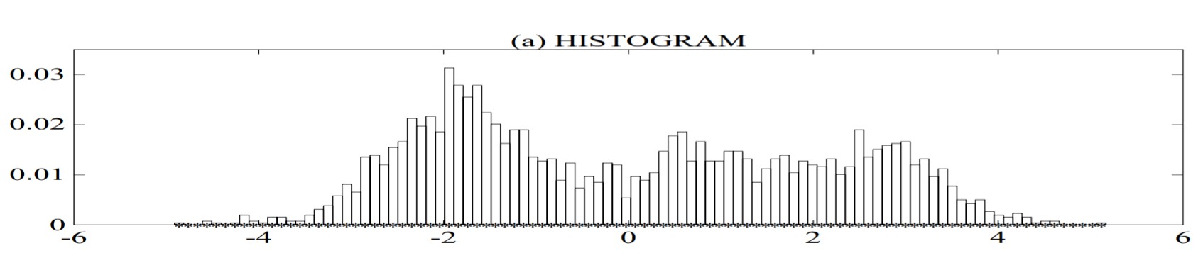
Plot (a) shows the histogram of a single feature from a speaker recognition system (a single cepstral value from a 25 second utterance by a male speaker);

graph

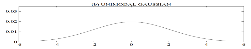
plot (b) shows a uni-modal Gaussian model of this feature distribution;

graph

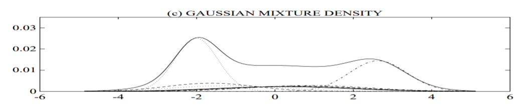
plot (c) shows a GMM and its ten underlying component densities; and

graph

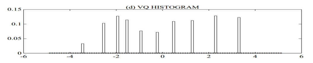
plot (d) shows a histogram of the data assigned to the VQ centroid locations of a 10 element codebook. The GMM not only provides a smooth overall distribution fit, its components also clearly detail the multi-modal nature of the density.

The use of a GMM for representing feature distributions in a biometric system may also be motivated by the intuitive notion that the individual component densities may model some underlying set of hidden classes. For example, in speaker recognition, it is reasonable to assume the acoustic space of spectral related features corresponding to a speaker’s broad phonetic events, such as vowels, nasals or fricatives. These acoustic classes reflect some general speaker dependent vocal tract configurations that are useful for characterizing speaker identity. The spectral shape of the ith acoustic class can in turn be represented by the mean µi of the ith component density, and variations of the average spectral shape can be represented by the covariance matrix Σi . Because all the features used to train the GMM are unlabeled, the acoustic classes are hidden in that the class of an observation is unknown. A GMM can also be viewed as a single-state HMM with a Gaussian mixture observation density, or an ergodic Gaussian observation HMM with fixed, equal transition probabilities. Assuming independent feature vectors, the observation density of feature vectors drawn from these hidden acoustic classes is a Gaussian mixture [2, 3].

Maximum Likelihood Parameter Estimation

Given training vectors and a GMM configuration, we wish to estimate the parameters of the GMM, λ, which in some sense best matches the distribution of the training feature vectors. There are several techniques available for estimating the parameters of a GMM. By far the most popular and well-established method is maximum likelihood (ML) estimation. The aim of ML estimation is to find the model parameters which maximize the likelihood of the GMM given the training data. For a sequence of T training vectors X = {x₁, . . . , x_T }, the GMM likelihood, assuming independence between the vectors1, can be written as,

$p\left ( X|\lambda\right )=\prod_{t=1}^{T}p\left ( X_{t}|\lambda \right )$ .

Unfortunately, this expression is a non-linear function of the parameters λ and direct maximization is not possible. However, ML parameter estimates can be obtained iteratively using a special case of the expectation-maximization (EM) algorithm [5]. The basic idea of the EM algorithm is, beginning with an initial model λ, to estimate a new model λ¯, such that p(X|λ¯) ≥ p(X|λ). The new model then becomes the initial model for the next iteration and the process is repeated until some convergence threshold is reached. The initial model is typically derived by using some form of binary VQ estimation. On each EM iteration, the following re-estimation formulas are used which guarantee a monotonic increase in the model’s likelihood value.

Mixture Weights

$\bar{\omega _{i}}= \frac{1}{T}\sum_{t=1}^{T}Pr\left ( i|X_{t},\lambda \right ),$

Means

$\bar{\mu _{i}}= \frac{\sum_{t=1}^{T}Pr\left ( i|X_{t},\lambda \right )X_{t}}{\sum_{t=1}^{T}Pr\left ( i|X_{t},\lambda \right )}.$

Variances (diagonal covariance)

$\bar{\sigma_{i}^{2}}= \frac{\sum_{t=1}^{T}Pr\left ( i|X_{t},\lambda \right )x_{t}^{2}}{\sum_{t=1}^{T}Pr\left ( i|X_{t},\lambda \right )}-\bar{\mu_{i}^{2}},$

The a posteriori probability for component i is given by

$Pr\left ( i|X_{t},\lambda \right )=\frac{\omega_{i}g\left ( X_{t}|\mu_{i},\sum _{i} \right )}{\sum_{k=1}^{M}\omega_{k}g\left ( X_{t}|\mu_{k},\sum _{k} \right )}$