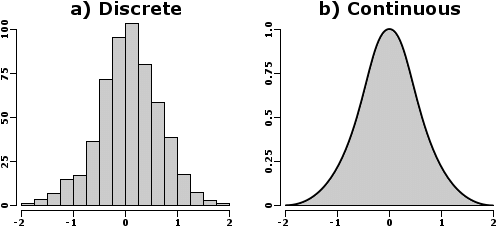
Discrete probability distributions
A discrete distribution describes the probability of occurrence of each value of a discrete random variable. A discrete random variable is a random variable that has countable values, such as a list of non-negative integers.
With a discrete probability distribution, each possible value of the discrete random variable can be associated with a non-zero probability. Thus, a discrete probability distribution is often presented in tabular form.
Example of the number of customer complaints
With a discrete distribution, unlike with a continuous distribution, you can calculate the probability that X is exactly equal to some value. For example, you can use the discrete Poisson distribution to describe the number of customer complaints within a day. Suppose the average number of complaints per day is 10 and you want to know the probability of receiving 5, 10, and 15 customer complaints in a day.
| x | P (X = x) |
|---|---|
| 5 | 0.037833 |
| 10 | 0.125110 |
| 15 | 0.034718 |
You can also view a discrete distribution on a distribution plot to see the probabilities between ranges.
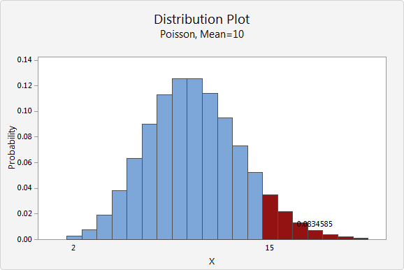
Distribution plot of the number of customer complaints
The shaded bars in this example represents the number of occurrences when the daily customer complaints is 15 or more. The height of the bars sums to 0.08346; therefore, the probability that the number of calls per day is 15 or more is 8.35%.
Several specialized discrete probability distributions are useful for specific applications. For business applications, three frequently used discrete distributions are:
- Binomial
- Geometric
- Poisson
You use the binomial distribution to compute probabilities for a process where only one of two possible outcomes may occur on each trial. The geometric distribution is related to the binomial distribution; you use the geometric distribution to determine the probability that a specified number of trials will take place before the first success occurs. You can use the Poisson distribution to measure the probability that a given number of events will occur during a given time frame.
Continuous probability distributions
A continuous distribution describes the probabilities of the possible values of a continuous random variable. A continuous random variable is a random variable with a set of possible values (known as the range) that is infinite and uncountable.
Probabilities of continuous random variables (X) are defined as the area under the curve of its PDF. Thus, only ranges of values can have a nonzero probability. The probability that a continuous random variable equals some value is always zero.
Example of the distribution of weights
The continuous normal distribution can describe the distribution of weight of adult males. For example, you can calculate the probability that a man weighs between 160 and 170 pounds.
However, the probability that X is exactly equal to some value is always zero because the area under the curve at a single point, which has no width, is zero. For example, the probability that a man weighs exactly 190 pounds to infinite precision is zero. You could calculate a nonzero probability that a man weighs more than 190 pounds, or less than 190 pounds, or between 189.9 and 190.1 pounds, but the probability that he weighs exactly 190 pounds is zero.
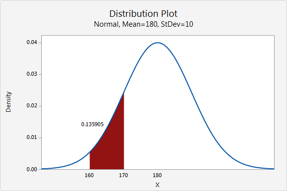
Distribution plot of the weight of adult males
The shaded region under the curve in this example represents the range from 160 and 170 pounds. The area of this range is 0.136; therefore, the probability that a randomly selected man weighs between 160 and 170 pounds is 13.6%. The entire area under the curve equals 1.0.
Many continuous distributions may be used for business applications; two of the most widely used are:
- Uniform
- Normal
The uniform distribution is useful because it represents variables that are evenly distributed over a given interval. For example, if the length of time until the next defective part arrives on an assembly line is equally likely to be any value between one and ten minutes, then you may use the uniform distribution to compute probabilities for the time until the next defective part arrives.
The normal distribution is useful for a wide array of applications in many disciplines. In business applications, variables such as stock returns are often assumed to follow the normal distribution. The normal distribution is characterized by a bell-shaped curve, and areas under this curve represent probabilities. The bell-shaped curve is shown here.
- Log in to post comments