Conditional probability is the probability of one event occurring with some relationship to one or more other events. For example:
- Event A is that it is raining outside, and it has a 0.3 (30%) chance of raining today.
- Event B is that you will need to go outside, and that has a probability of 0.5 (50%).
A conditional probability would look at these two events in relationship with one another, such as the probability that it is both raining and you will need to go outside.
Conditional probability is the probability of a particular event Y, given a certain condition which has already occurred , i.e., X. Then conditional probability, P(Y|X) is defined as,
P(Y|X) = N(X∩Y) / N(X); provide N(X) > 0
N(X): – Total cases favourable to the event X
N(X∩Y): – Total favourable simultaneous
Or, we can write as:
P(Y|X) = P(X∩Y) / P(X); P(X) > 0
Independent, Dependent and Exclusive Events
Assume we have two events – Event A and Event B.
On the off chance that the occurring of event A doesn’t influence the occurring of event B, these events are called as independent events.
Let’s explore few cases of independent events:
- Getting heads subsequent to flipping a coin AND getting a 5 on throw of a fair die.
- Choosing a marble from a container AND getting heads in the flipping of a coin.
- Choosing a 3 card from a deck of cards, placing it back, AND then picking an ace as the second card.
- Rolling a 4 on a reasonable throw of a fair die, AND then rolling a 1 on another die.
In each of these cases the probability of result of the second event isn’t influenced at all by the result of the first event.
Probability of independent events
For this situation the probability of P (A ꓵ B) = P (A) * P (B)
We will take a case here for better understanding. Assume we win the challenge, if we pick a red marble from a jug containing 4 red and 3 dark marbles and we get heads on the flip of a coin. What is the probability of winning?
We characterize event A, as getting red marble from the jug.
Event B is getting heads on the flip of a coin.
We have to discover the probability of both, getting a red marble and a heads in a coin toss.
P (A) = 4/7
P (B) = 1/2
We realize that there is no effect of the marble color on the result of the coin toss.
P (A ꓵ B) = P (A) * P (B)
P (A ꓵ B) = (4/7) * (1/2) = (2/7)
Probability of dependent events
Next, think about the cases of dependent events?
In the above case, we characterize event A as getting a Red marble from the jug. We at that point keep the marble out and after that take another marble from the jug.
Mutually exclusive and exhaustive events
Mutually exclusive events are those events where two events can’t occur together.
The most straightforward case to comprehend this is the flip of a coin. Getting a head and a tail are mutually exclusive on the grounds that we can either get heads or tails but never both at the same time in one single coin toss.
An arrangement of events is on the whole exhaustive when the set ought to contain all the possible results of the trial. One of the events from the set must happen surely when the experiment is done.
For instance, in a fair die throw, {1,2,3,4,5,6} is an exhaustive collection since it includes the whole scope of the achievable outcomes.
Consider the results “even” (2,4 or 6) and “not-6” (1,2,3,4, or 5) in a throw of a fair die. They are collectively exhaustive but if you observe closely they aren’t mutually exclusive.
Bayes Theorem of Conditional Probability
Before we dive into Bayes theorem, let’s review marginal, joint, and conditional probability.
Recall that marginal probability is the probability of an event, irrespective of other random variables. If the random variable is independent, then it is the probability of the event directly, otherwise, if the variable is dependent upon other variables, then the marginal probability is the probability of the event summed over all outcomes for the dependent variables, called the sum rule.
- Marginal Probability: The probability of an event irrespective of the outcomes of other random variables, e.g. P(A).
The joint probability is the probability of two (or more) simultaneous events, often described in terms of events A and B from two dependent random variables, e.g. X and Y. The joint probability is often summarized as just the outcomes, e.g. A and B.
- Joint Probability: Probability of two (or more) simultaneous events, e.g. P(A and B) or P(A, B).
The conditional probability is the probability of one event given the occurrence of another event, often described in terms of events A and B from two dependent random variables e.g. X and Y.
- Conditional Probability: Probability of one (or more) event given the occurrence of another event, e.g. P(A given B) or P(A | B).
The joint probability can be calculated using the conditional probability; for example:
- P(A, B) = P(A | B) * P(B)
This is called the product rule. Importantly, the joint probability is symmetrical, meaning that:
- P(A, B) = P(B, A)
The conditional probability can be calculated using the joint probability; for example:
- P(A | B) = P(A, B) / P(B)
The conditional probability is not symmetrical; for example:
- P(A | B) != P(B | A)
An Alternate Way To Calculate Conditional Probability
Now, there is another way to calculate the conditional probability.
Specifically, one conditional probability can be calculated using the other conditional probability; for example:
- P(A|B) = P(B|A) * P(A) / P(B)
The reverse is also true; for example:
- P(B|A) = P(A|B) * P(B) / P(A)
This alternate approach of calculating the conditional probability is useful either when the joint probability is challenging to calculate (which is most of the time), or when the reverse conditional probability is available or easy to calculate.
This alternate calculation of the conditional probability is referred to as Bayes Rule or Bayes Theorem, named for Reverend Thomas Bayes, who is credited with first describing it. It is grammatically correct to refer to it as Bayes’ Theorem (with the apostrophe), but it is common to omit the apostrophe for simplicity.
- Bayes Theorem: Principled way of calculating a conditional probability without the joint probability.
It is often the case that we do not have access to the denominator directly, e.g. P(B).
We can calculate it an alternative way; for example:
- P(B) = P(B|A) * P(A) + P(B|not A) * P(not A)
This gives a formulation of Bayes Theorem that we can use that uses the alternate calculation of P(B), described below:
- P(A|B) = P(B|A) * P(A) / P(B|A) * P(A) + P(B|not A) * P(not A)
Or with brackets around the denominator for clarity:
- P(A|B) = P(B|A) * P(A) / (P(B|A) * P(A) + P(B|not A) * P(not A))
Note: the denominator is simply the expansion we gave above.
As such, if we have P(A), then we can calculate P(not A) as its complement; for example:
- P(not A) = 1 – P(A)
Additionally, if we have P(not B|not A), then we can calculate P(B|not A) as its complement; for example:
- P(B|not A) = 1 – P(not B|not A)
Naming the Terms in the Theorem
The terms in the Bayes Theorem equation are given names depending on the context where the equation is used.
It can be helpful to think about the calculation from these different perspectives and help to map your problem onto the equation.
Firstly, in general, the result P(A|B) is referred to as the posterior probability and P(A) is referred to as the prior probability.
- P(A|B): Posterior probability.
- P(A): Prior probability.
Sometimes P(B|A) is referred to as the likelihood and P(B) is referred to as the evidence.
- P(B|A): Likelihood.
- P(B): Evidence.
This allows Bayes Theorem to be restated as:
- Posterior = Likelihood * Prior / Evidence
We can make this clear with a smoke and fire case.
What is the probability that there is fire given that there is smoke?
Where P(Fire) is the Prior, P(Smoke|Fire) is the Likelihood, and P(Smoke) is the evidence:
- P(Fire|Smoke) = P(Smoke|Fire) * P(Fire) / P(Smoke)
You can imagine the same situation with rain and clouds.
Now that we are familiar with Bayes Theorem and the meaning of the terms, let’s look at a scenario where we can calculate it.
Worked Example for Calculating Bayes Theorem
Bayes theorem is best understood with a real-life worked example with real numbers to demonstrate the calculations.
First we will define a scenario then work through a manual calculation, a calculation in Python, and a calculation using the terms that may be familiar to you from the field of binary classification.
- Diagnostic Test Scenario
- Manual Calculation
- Python Code Calculation
- Binary Classifier Terminology
Let’s go.
Diagnostic Test Scenario
An excellent and widely used example of the benefit of Bayes Theorem is in the analysis of a medical diagnostic test.
Scenario: Consider a human population that may or may not have cancer (Cancer is True or False) and a medical test that returns positive or negative for detecting cancer (Test is Positive or Negative), e.g. like a mammogram for detecting breast cancer.
Problem: If a randomly selected patient has the test and it comes back positive, what is the probability that the patient has cancer?
Manual Calculation
Medical diagnostic tests are not perfect; they have error.
Sometimes a patient will have cancer, but the test will not detect it. This capability of the test to detect cancer is referred to as the sensitivity, or the true positive rate.
In this case, we will contrive a sensitivity value for the test. The test is good, but not great, with a true positive rate or sensitivity of 85%. That is, of all the people who have cancer and are tested, 85% of them will get a positive result from the test.
- P(Test=Positive | Cancer=True) = 0.85
Given this information, our intuition would suggest that there is an 85% probability that the patient has cancer.
Our intuitions of probability are wrong.
This type of error in interpreting probabilities is so common that it has its own name; it is referred to as the base rate fallacy.
It has this name because the error in estimating the probability of an event is caused by ignoring the base rate. That is, it ignores the probability of a randomly selected person having cancer, regardless of the results of a diagnostic test.
In this case, we can assume the probability of breast cancer is low, and use a contrived base rate value of one person in 5,000, or (0.0002) 0.02%.
- P(Cancer=True) = 0.02%.
We can correctly calculate the probability of a patient having cancer given a positive test result using Bayes Theorem.
Let’s map our scenario onto the equation:
- P(A|B) = P(B|A) * P(A) / P(B)
- P(Cancer=True | Test=Positive) = P(Test=Positive|Cancer=True) * P(Cancer=True) / P(Test=Positive)
We know the probability of the test being positive given that the patient has cancer is 85%, and we know the base rate or the prior probability of a given patient having cancer is 0.02%; we can plug these values in:
- P(Cancer=True | Test=Positive) = 0.85 * 0.0002 / P(Test=Positive)
We don’t know P(Test=Positive), it’s not given directly.
Instead, we can estimate it using:
- P(B) = P(B|A) * P(A) + P(B|not A) * P(not A)
- P(Test=Positive) = P(Test=Positive|Cancer=True) * P(Cancer=True) + P(Test=Positive|Cancer=False) * P(Cancer=False)
Firstly, we can calculate P(Cancer=False) as the complement of P(Cancer=True), which we already know
- P(Cancer=False) = 1 – P(Cancer=True)
- = 1 – 0.0002
- = 0.9998
Let’s plugin what we have:
We can plug in our known values as follows:
- P(Test=Positive) = 0.85 * 0.0002 + P(Test=Positive|Cancer=False) * 0.9998
We still do not know the probability of a positive test result given no cancer.
This requires additional information.
Specifically, we need to know how good the test is at correctly identifying people that do not have cancer. That is, testing negative result (Test=Negative) when the patient does not have cancer (Cancer=False), called the true negative rate or the specificity.
We will use a contrived specificity value of 95%.
- P(Test=Negative | Cancer=False) = 0.95
With this final piece of information, we can calculate the false positive or false alarm rate as the complement of the true negative rate.
- P(Test=Positive|Cancer=False) = 1 – P(Test=Negative | Cancer=False)
- = 1 – 0.95
- = 0.05
We can plug this false alarm rate into our calculation of P(Test=Positive) as follows:
- P(Test=Positive) = 0.85 * 0.0002 + 0.05 * 0.9998
- P(Test=Positive) = 0.00017 + 0.04999
- P(Test=Positive) = 0.05016
Excellent, so the probability of the test returning a positive result, regardless of whether the person has cancer or not is about 5%.
We now have enough information to calculate Bayes Theorem and estimate the probability of a randomly selected person having cancer if they get a positive test result.
- P(Cancer=True | Test=Positive) = P(Test=Positive|Cancer=True) * P(Cancer=True) / P(Test=Positive)
- P(Cancer=True | Test=Positive) = 0.85 * 0.0002 / 0.05016
- P(Cancer=True | Test=Positive) = 0.00017 / 0.05016
- P(Cancer=True | Test=Positive) = 0.003389154704944
The calculation suggests that if the patient is informed they have cancer with this test, then there is only 0.33% chance that they have cancer.
It is a terrible diagnostic test!
The example also shows that the calculation of the conditional probability requires enough information.
For example, if we have the values used in Bayes Theorem already, we can use them directly.
This is rarely the case, and we typically have to calculate the bits we need and plug them in, as we did in this case. In our scenario we were given 3 pieces of information, the the base rate, the sensitivity (or true positive rate), and the specificity (or true negative rate).
- Sensitivity: 85% of people with cancer will get a positive test result.
- Base Rate: 0.02% of people have cancer.
- Specificity: 95% of people without cancer will get a negative test result.
We did not have the P(Test=Positive), but we calculated it given what we already had available.
We might imagine that Bayes Theorem allows us to be even more precise about a given scenario. For example, if we had more information about the patient (e.g. their age) and about the domain (e.g. cancer rates for age ranges), and in turn we could offer an even more accurate probability estimate.
Conditional Probability in Real Life
Conditional probability is used in many areas, in fields as diverse as calculus, insurance, and politics. For example, the re-election of a president depends upon the voting preference of voters and perhaps the success of television advertising—even the probability of the opponent making gaffes during debates!
The weatherman might state that your area has a probability of rain of 40 percent. However, this fact is conditional on many things, such as the probability of…
- …a cold front coming to your area.
- …rain clouds forming.
- …another front pushing the rain clouds away.
We say that the conditional probability of rain occurring depends on all the above events.
Where does the Conditional Probability Formula Come From?
The formula for conditional probability is derived from the probability multiplication rule, P(A and B) = P(A)*P(B|A). You may also see this rule as P(A∪B). The Union symbol (∪) means “and”, as in event A happening and event B happening.
Step by step, here’s how to derive the conditional probability equation from the multiplication rule:
Step 1: Write out the multiplication rule:
P(A and B) = P(A)*P(B|A)
Step 2: Divide both sides of the equation by P(A):
P(A and B) / P(A) = P(A)*P(B|A) / / P(A)
Step 3: Cancel P(A) on the right side of the equation:
P(A and B) / P(A) = P(B|A)
Step 4: Rewrite the equation:
P(B|A) = P(A and B) / P(A)
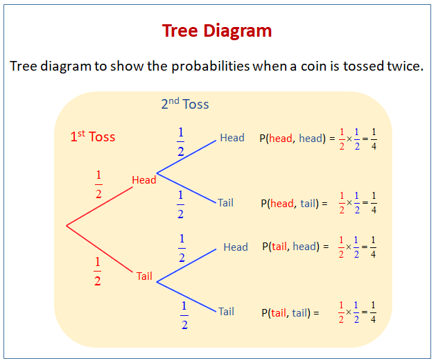
Conditional probabilities can be found using a tree diagram. In the tree diagram, the probabilities in each branch are conditional.
Conditional Probability for Independent Events
Two events are independent if the probability of the outcome of one event does not influence the probability of the outcome of another event. Due to this reason, the conditional probability of two independent events A and B is:
P(A|B) = P(A)
P(B|A) = P(B)
Conditional Probability for Mutually Exclusive Events
In probability theory, mutually exclusive events are events that cannot occur simultaneously. In other words, if one event has already occurred, another can event cannot occur. Thus, the conditional probability of mutually exclusive events is always zero.
P(A|B) = 0
P(B|A) = 0
Data Science and Conditional Probability
Data Science often uses statistical inferences to predict or analyze trends from data, while statistical inferences make use of probability distributions of data. Therefore, knowing probability and its applications are important to work effectively on data science problems.
Most data science techniques rely on Bayes’ theorem. Bayes’ theorem is a formula that describes at large how to update the probabilities of hypotheses when given evidence. You can build a learner using the Bayes’ theorem to predicts the probability of the response variable belonging to some class, given a new set of attributes.
Data Science is inextricably linked to Conditional Probability. Data Science professionals must have a thorough understanding of probability to solve complicated data science problems. A strong base in Probability and Conditional Probability is essential to fully understand and implement relevant algorithms for use.
Data Science & Conditional Probability
Do you aspire to be a Data Analyst, and then grow further to become a Data Scientist? Do you like finding answers to complex business challenges interests? Whatever you want, start early to gain a competitive advantage. You must be fluent in the programming languages and tools that will help you get hired.
You may also read my earliest post on How to Create a Killer Data Analyst Resume to create winning CVs that will leave an impression in the mind of the recruiters.
You may start as a Data Analyst, go on to become a Data Scientist with some years of experience, and eventually a data evangelist. Data Science offers lucrative career options. There is enough scope for growth and expansion.
You might be a programmer, a mathematics graduate, or simply a bachelor of Computer Applications. Students with a master’s degree in Economics or Social Science can also be a data scientist. Take up a Data Science or Data Analytics course, to learn Data Science skills and prepare yourself for the Data Scientist job, you have been dreaming of.
- Log in to post comments