Best Fit Line

"A line that is drawn to pass as close as possible to all the plotted points on a scatter graph is called the line of best fit"

best fit line

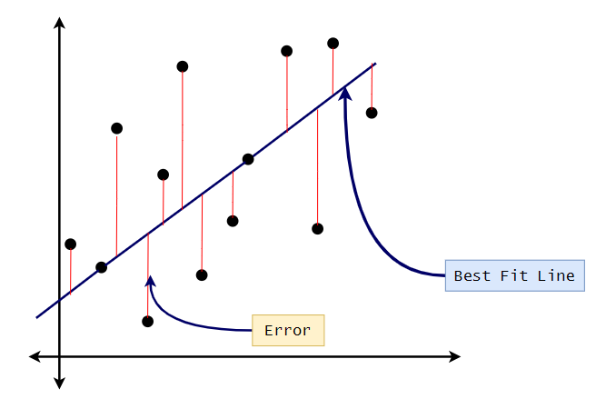
we cannot plot a single straight line that passes through all the points. So what we can do here is to minimize the error. It means that we find a bar and then find the prediction error. Since we have the actual value here, we can easily find the error in prediction. Our ultimate goal will be to find the line that has the minimal error. That line is called the linear best fit. When there are more than 2 points of data it is usually impossible to find a line that goes exactly through all the points. But, usually we can find a line (or curve) that is a good approximation to the data. It is important for us to keep our numbers straight, so we have created a few variables below which we defined to the right.

The line for which the the error between the predicted values and the observed values is minimum is called the best fit line or the regression line. These errors are also called as residuals. The residuals can be visualized by the vertical lines from the observed data value to the regression line.

When there are more than 2 points of data it is usually impossible to find a line that goes exactly through all the points. But, usually we can find a line (or curve) that is a good approximation to the data.

The best form for our line is slope-intercept form, which looks like y = mx + b. Therefore, it is only necessary to compute m and b to determine the best fit line. Those values can be computed by the following equations:

$m = \frac{(N\sum xy) - (\sum x\sum y)}{(N\sum x^{2}) - (\sum x\sum x)}$

$b = \frac{(\sum x^{2} \sum y) - (\sum x\sum xy)}{(N\sum x^{2}) - (\sum x\sum x)}$

$\sum x$ - The sum of all the values in the x column.

$\sum y$ - The sum of all the values in the y column.

$\sum xy$ - The sum of the products of the x_n and y_n that are recorded at the same time.

$\sum x^{2}$ - The total of each value in the x column squared and then added together.

$\sum y^{2}$ - The total of each value in the y column squared and then added together.

N - The total number of elements (or trials in your experiment).

For our example, here's how you would calculate these:

x	4.1	6.5	12.6	25.5	29.8	38.6	46	52.8	59.6	66.3	74.7
y	2.2	4.5	10.4	23.1	27.9	36.8	44.3	50.7	57.5	64.1	72.6

x_sum = 4.1 + 6.5 + 12.6 + 25.5 + 29.8 + 38.6 + 46 + 52.8 + 59.6 + 66.3 + 74.7 = 416.5

y_sum = 2.2 + 4.5 + 10.4 + 23.1 + 27.9 + 36.8 + 44.3 + 50.7 + 57.5 + 64.1 + 72.6 = 394.1

xy_sum = 4.1*2.2 + 6.5*4.5 + 12.6*10.4 + 25.5*23.1 + 29.8*27.9 + 38.6*36.8 + 46*44.3 + 52.8*50.7 + 59.6*57.5 + 66.3*64.1 + 74.7*72.6 = 20825

x²_sum = 4.1² + 6.5² + 12.6² + 25.5² + 29.8² + 38.6² + 46² + 52.8² + 59.6² + 66.3² + 74.7² = 21678

y²_sum = 2.2² + 4.5² + 10.4² + 23.1² + 27.9² + 36.8² + 44.3² + 50.7² + 57.5² + 64.1² + 72.6² = 20018

N = 11

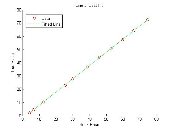
After plugging in the values that we found, we get: m = .99992 and b = -2.0067.

This means that the equation of the line is y = .99992x + -2.0067, or y = .99992x - 2.0067. We graphed the results using Matlab, but you can even make a graph by hand.

best fit line

OR

Line of Best Fit (Least Square Method): A line of best fit is a straight line that is the best approximation of the given set of data.

It is used to study the nature of the relation between two variables. (We're only considering the two-dimensional case, here.)

A line of best fit can be roughly determined using an eyeball method by drawing a straight line on a scatter plot so that the number of points above the line and below the line is about equal (and the line passes through as many points as possible).

A more accurate way of finding the line of best fit is the least square method. Use the following steps to find the equation of line of best fit for a set of ordered pairs.

(x₁,y₁),(x₂,y₂),...,(x_n,y_n)

Step 1: Calculate the mean of the x -values and the mean of the y -values.

$\bar{X} = \frac{\sum_{i=1}^{n}x_{i}}{n}, \bar{Y} = \frac{\sum_{i=1}^{n}y_{i}}{n}$

Step 2: The following formula gives the slope of the line of best fit:

$m = \frac{\sum_{i=1}^{n}\left ( x_{i}-\bar{X}\right )\left ( y_{i}-\bar{Y} \right )}{\left ( x_{i}-\bar{X}\right )}$

Step 3: Compute the y -intercept of the line by using the formula:

$b = \bar{Y} - m\bar{X}$

Step 4: Use the slope m and the y -intercept bb to form the equation of the line.

Example:

Use the least square method to determine the equation of line of best fit for the data. Then plot the line.

x	8	2	11	6	5	4	12	9	6	1
y	3	10	3	6	8	12	1	4	9	14

Solution:

best fit line

Calculate the means of the x -values and the y -values.

$\bar{X} = \frac{8 + 2 + 11 + 6 + 5 + 4 + 12 + 9 + 6 + 1}{10} = 6.4$

Now calculate $x_{i}-\bar{X}$ , $y_{i}-\bar{Y}$ , $(x_{i}-\bar{X})$ $(y_{i}-\bar{Y})$ and $(x_{i}-\bar{X})^{2}$ for each i.

i	x_i	y_i	$x_{i}-\bar{X}$	$y_{i}-\bar{Y}$	$(x_{i}-\bar{X})$ $(y_{i}-\bar{Y})$	$(x_{i}-\bar{X})^{2}$
1	8	3	1.6	−4	−6.4	2.56
2	2	10	−4.4	3	−13.2	19.36
3	1	3	4.6	−4	−18.4	21.16
4	6	6	−0.4	−1	0.4	0.16
5	5	8	−1.4	1	−1.4	1.96
6	4	12	−2.4	5	−12	5.76
7	12	1	5.6	−6	−33.6	31.36
8	9	4	2.6	−3	−7.8	6.76
9	6	9	−0.4	2	−0.8	0.16
10	1	14	−5.4	7	−37.8	29.16
					$\sum_{i=1}^{n}(x_{i}-\bar{X})(y_{i}-\bar{Y})=-131$	$\sum_{i=1}^{n}(x_{i}-\bar{X})^{2}=118.4$

Calculate the slope.

$m = \frac{\sum_{i=1}^{n}(x_{i}-\bar{X})(y_{i}-\bar{Y})}{\sum_{i=1}^{n}(x_{i}-\bar{X})^{2}} = \frac{-131}{118.4} \approx -1.1$

Calculate the y -intercept.

Use the formula to compute the y -intercept.

$b=\bar{Y}-m\bar{X}=7-\left ( -1.1\times 6.4 \right )=7+6.4\approx 14.0$

Use the slope and y -intercept to form the equation of the line of best fit.

The slope of the line is −1.1 and the y -intercept is 14.0 .

Therefore, the equation is y = −1.1x + 14.0,

Draw the line on the scatter plot.

best fit line

Why (and when) should I use a best fit line?

In introductory geoscience, most exercises that ask you to construct a best-fit line have to do with wanting to be able recognize relationships among variables on Earth or to predict the behavior of a system (in this case the Earth system). We want to know if there is a relationship between the amount of nitrogen in the water and the intensity of an algal bloom, or we wish to know the relationship of one chemical component of a rock to another. For predictive purposes, we might prefer to know how often an earthquake is likely to occur on a particular fault or the possibility of a very large flood on a given river. All of these applications use best-fit lines on scatter plots (x-y graphs with just data points, no lines).

If you find yourself faced with a question that asks you to draw a trend line, linear regression or best-fit line, you are most certainly being asked to draw a line through data points on a scatter plot. You may also be asked to approximate the trend, or sketch in a line that mimics the data. This page is designed to help you complete any of these types of questions. Work through it and the sample problems if you are unsure of how to complete questions about trends and best-fit lines.